Neural Belief Propagation Auto-Encoder for Linear Block Code Design
Orange Institut Polytechnique de Paris
September 21, 2022
IEEE Transactions on Communications - 10.1109/TCOMM.2022.3208331
Copyright Notice: 2022 IEEE. Personal use of this material is permitted. Permission from IEEE must be obtained for all other uses, in any current or future media, including reprinting/republishing this material for advertising or promotional purposes, creating new collective works, for resale or redistribution to servers or lists, or reuse of any copyrighted component of this work in other works.
This work has been partly funded by the European Commission through the H2020 project Hexa-X (Grant Agreement no. 101015956).
Abstract
The growing number of Internet of Thing (IoT) and Ultra-Reliable Low Latency Communications (URLCC) use cases in next generation communication networks calls for the development of efficient Forward Error Correction (FEC) mechanisms. These use cases usually imply using short to mid-sized information blocks and requires low-complexity and/or fast decoding procedures. This paper investigates the joint learning of short to mid block-length coding schemes and associated Belief-Propagation (BP) like decoders using Machine Learning (ML) techniques. An interpretable auto-encoder (AE) architecture is proposed, ensuring scalability to block sizes currently challenging for ML-based linear block code design approaches. By optimizing a coding scheme w.r.t. the targeted decoder, the proposed system offers a good complexity/performance trade-off compared to various codes from literature with length up to 128 bits.
Introduction
Efficient Forward Error Correction (FEC) schemes are a key enabler for Internet of Things (IoT) scenarios and/or Ultra-Reliable Low Latency Communications (URLLC). Such use-cases typically imply the use of short packets and low-complexity and/or fast (de)coding schemes, in line with latency, energy consumption, hardware cost and computational power constraints. Existing FEC codes, such as Bose Chaudhuri and Hocquenghem (BCH), TB-CC, Turbo, Polar or Low Density Parity Check (LDPC) codes, and their respective decoders, attempt to meet these needs, each with their own advantages and limitations. In late 2018, 3GPP agreed to use Polar codes for the control channels and LDPC for the data channels of the 5G-NR interface for enhanced Mobile Broad-Band (eMBB) applications [1]. On the one hand, for high throughput applications, large LDPC codes offer near capacity performances, efficient encoding and decoding with highly parallel decoders based on Belief Propagation (BP) and variants, e.g. Min-Sum (MS) [2] or Offset Min-Sum (OMS) [3]. On the other hand, Polar codes are proven to achieve capacity on Binary Symetric Channel (BSC) and offer a reasonable decoding complexity for shorter block lengths based on successive cancellation list decoders. While BP decoders offer high performance and efficient decoding for long and sparse codes, they tend to be less efficient for decoding smaller, usually denser, ones. Similarly, successive cancellation list decoders offer high performance and low decoding complexity for short codes, but they tend to become inapplicable when considering larger codes. Therefore, there is currently no efficient unified Linear Block Code (LBC) decoder architecture for all code lengths and rate ranges. Such an architecture would be of great interest for next generation communication networks such as 6th Generation (6G) networks. Different research directions can be explored to achieve this goal, among which the improvement of the performance of BP-like decoders and/or the design of better codes for such decoders to extend their use to shorter block lengths. This option has certain advantages. In particular, BP decoders were, to some extent, originally designed for low complexity decoding of long blocks. Such scalability is particularly difficult to satisfy when designing a new decoding algorithm and the BP therefore appears to be a judicious starting point. In addition, some work in the literature has started to explore this direction and some interesting initial results have been published [4], [5], [6], [7], [8].
Artificial Intelligence (AI) and Machine Learning (ML) techniques are deemed to play a major role in 6G networks [9], [10] and they have naturally been applied to the field of channel coding and particularly to the short block length regime. Multiple contributions have succeeded in improving the decoding performance by applying a Neural Network (NN)-based decoder to an existing coding scheme. One such example is the work on Neural Belief Propagation (NBP), which seeks to implement a trainable weighted BP decoder to improve the decoding performance of short BCH codes [4]. Following this idea, similar approaches are employed in [5], [6], [7], [8], [11]. Other contributions try to learn an End-to-End (E2E) communication schemes, including channel coding. As an example, an Auto-Encoder (AE) NN models is used in [12] to jointly design the transmitter and receiver of a simple communication scheme. However, while interesting, these E2E black-box approaches are, to the best of the authors knowledge, currently limited to, either small code sizes, e.g. (8,4) or (15,7) in [12], or rely on extremely large models, particularly complex to train notably because of the so called “Curse of dimensionality”. This well-known phenomenon in ML is related to the fact that the solution space of a problem grows exponentially with its dimensionality. This makes the available training data sparse and thus non-statistically significant or the needed volume of training samples too important. Similarly, the “Curse of (code-word) dimensionality” appears in the context of Physical (PHY) layer when one tries to train models with increased information block sizes. The number of code-words associated to information blocks of size \(k\) is of \(2^k\) which can rapidly become prohibitively large when increasing \(k\), making the learning of large codes a challenging problem [9], [12].
To alleviate this problem, one solution is to use structured approaches [13], [14], [15], [16], p 576-577. One can for example exploit code structures such as convolutional codes [17] or construct specific NN-based decoder structure using Recurrent Neural Network (RNN) [18] or Convolutional Neural Network (CNN) [17] to circumvent this dimensionality problem. Still, existing approaches are, to the best of the authors knowledge, limited to the design of convolutional [17], [18], Turbo [19] or Polar codes [20] and often exhibit a high number of model parameters and a reduced interpretability. Also, the comparison with traditional (de)coding schemes is sometimes complex. Indeed, the proposed solutions are often based on the learning of E2E communication schemes (usually based on AE), not limited to the (de)coding function but also allow the joint learning of (de)modulation, equalization, etc. It then becomes difficult to distinguish the contribution of each of these functions to the final performance in view of a fair comparison with classical approaches. A different approach based on BP decoders uses a Genetic Algorithm (GA) to optimize LDPC codes from existing distributions with promising results [21].
In a previous work [11], a low-complexity, generic, NN-based BP decoder called Gated Neural Belief Propagation (GNBP) that learns to decode a LBC without prior knowledge of the coding scheme used at the transmitter was proposed. In this paper, an interpretable AE system able to jointly design a LBC and its associated GNBP decoder offering a competitive level of performance with low computational complexity is proposed. Instead of using ML techniques to improve the performance of decoders (e.g. BP) on codes from the literature that are flawed w.r.t. the latters (e.g. BCH codes), this paper proposes to jointly design short codes performing well w.r.t. the targeted BP decoder. This approach is to some extent comparable to that of [20] which uses ML to design performing Polar codes w.r.t. a differentiable BP decoder. The main objectives of the study are to propose a low-complexity structured approach that offers good performance, scalability and interpretability while making no assumptions about the code structure.
The reader is referred to [16] for detailed explanations on NN models and related optimization algorithms based on Gradient Descent (GD) used in this publication.
This paper uses the following notations: scalars are denoted as \(s\), line vectors as \(\mathbf{v}\) and matrices as \(\mathbf{M}\). \(\mathbf{M}^{n,m}\) is a matrix of size \(n\) by \(m\). \(\mathbf{M}^T\) is the transpose of \(\mathbf{M}\). \(\mathbb{F}_2\) is the binary finite field.
Theoretical Background
Linear Block Codes and Associated Graphical Representations
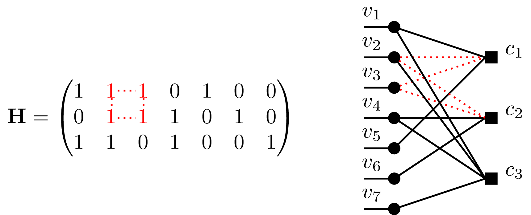
LBC are a class of FECs for which the information to be transmitted is split into blocks of fixed size \(k\) named words. Words are encoded using linear combinations to form code-words of size \(n\) with \(n > k\). Let \(\mathcal{C}(n,k)\) be a binary LBC of length \(n\) and rank \(k\) that will be referred to as an “\((n,k)\) code” throughout this paper. Let \(\mathbf{G} \in \mathbb{F}_2^{k,n}\) be the associated generator matrix of size \(k\) by \(n\) describing the encoding relations. Let \(\mathbf{H} \in \mathbb{F}_2^{(n-k),n}\) be the corresponding Parity-Check (PC) matrix of size \((n-k)\) by \(n\) constructed such that \(\mathbf{G}\mathbf{H}^T = \mathbf{0} \: \in \mathbb{F}_2^{k,(n-k)}\). The encoding process to obtain a code-word \(\mathbf{c} \in \mathbb{F}_2^n\) from a word \(\mathbf{x} \in \mathbb{F}_2^k\) is defined as \(\mathbf{c} = \mathbf{x}\mathbf{G}\). Using linear combinations of the rows and columns permutations, a standard form of the generator matrix \(\mathbf{G}_\mathrm{std} = \left( \mathbf{I}^{k,k} | \mathbf{R}^{k,(n-k)}\right)\) can be obtained, where \(\mathbf{I}^{k,k}\) and \(\mathbf{R}^{k,(n-k)}\) are respectively an identity matrix and a redundancy matrix. Using the standard form results in a simplified encoding process with code-words of the form \(\mathbf{c} = (\mathbf{x}|\mathbf{r})\) where \(\mathbf{x}\) is the raw information word and \(\mathbf{r}\) the computed redundancy. The code is then said to be systematic. When \(\mathbf{G}\) is in the standard form, the corresponding PC can simply be obtained as \(\mathbf{H}_\mathrm{std} = \left(\left[\mathbf{R}^{k,(n-k)}\right]^T \left| \mathbf{I}^{(n-k),(n-k)} \right.\right)\).
A bipartite graphical representation called a Tanner Graph (TG) [22] can be used to describe any PC matrix (Fig. 1). The check nodes connections represent the rows of the matrix and the variable nodes connections the columns. Following notations from [23], a convenient way to describe LBC ensembles and particularly LDPC ensembles is to use degree distribution pairs \((\Lambda,P)\). Let the degree of a node be its number of edges. Let \(\Lambda_i\) be the number of variable nodes with degree \(i\) and \(P_j\) be the number of check nodes with degree \(j\). From these notations, one can define the variable and check degree distribution from node perspective polynomials: \[\left\{ \begin{aligned} \Lambda(x) = \sum_i \Lambda_i x^i \\ P(x) = \sum_j P_j x^j \\ \end{aligned} \right.\] The normalized degree distributions from node perspective are written as: \[\left\{ \begin{aligned} &L(x) = \frac{\Lambda(x)}{\Lambda(1)} = \sum_i \frac{\Lambda_ix^i}{\Lambda(1)} = \sum_i L_i x^i\\ &R(x) = \frac{P(x)}{P(1)} = \sum_j \frac{P_jx^j}{P(1)} = \sum_j R_j x^j\\ \end{aligned} \right.\] where \(\Lambda(1)\) and \(P(1)\) are respectively the total number of variable and check nodes. In other words, \(L_i\) and \(R_j\) are respectively the probability that a variable and a check node chosen uniformly at random among the \(n\) and \((n-k)\) nodes has a degree \(i\) and \(j\).
Belief Propagation Decoders and Variants
Belief Propagation Decoder1
TG representations enable efficient iterative decoding based on message-passing algorithms such as the BP. In the context of communication systems, messages exchanged at the decoder between the nodes of the TG are usually related to the Log-Likelihood Ratio (LLR) of transmitted bits. The Sum-Product (SP) update rule can be applied iteratively to the nodes of a code graph using equations [eq:sum], [eq:product] and [eq:out] (see [24] for the detailed derivations). Message from the variable node \(i\) toward the check node \(j\) is computed using: \[\mu_{v_i \xrightarrow[]{} c_j} = \lambda_i + \sum_{l \neq j}{\mu_{c_l \xrightarrow[]{} v_i}} \label{eq:sum}\] where \(\lambda_i\) is the a priori LLR received by variable node \(i\) and \(\mu_{c_l \xrightarrow[]{} v_i}\) are the other messages received by variable node \(i\) from neighboring check nodes \(l\).
Similarly, message from the check node \(j\) toward the variable node \(i\) is defined as: \[\mu_{c_j \xrightarrow[]{} v_i} = 2\:\mathrm{artanh} \left[ \prod_{l \neq i} \mathrm{tanh}\left(\frac{\mu_{v_l \xrightarrow[]{} c_j}}{2}\right)\right] \label{eq:product}\] where \(\mu_{v_l \xrightarrow[]{} c_j}\) are the messages received by check node \(j\) from neighboring variable nodes \(l\).
Finally, the a posteriori LLR can be computed at the variable node \(i\) as: \[\widetilde{\lambda_i} = \lambda_i + \sum_{l}{\mu_{c_l \xrightarrow[]{} v_i}} \label{eq:out}\] BP is generally exact for tree structures (meaning that it always converges to the true posterior in one pass) but only approximate for graphs with cycles. The presence of such loops in the inference graph can induce undesirable feedback effects (see Fig. 1). The TG of codes are generally not cycle-free and the BP inference not exact, hence the necessity to apply iterative decoding by passing messages back and forth between variable and check nodes, using equations [eq:sum] and [eq:product], before hopefully converging to a satisfying solution. In practice, the BP has proven to be effective in the decoding of high girth (the shortest cycle of a TG) codes, such as large LDPC, offering both high performance and reasonable complexity. For shorter and higher density codes, the presence of short cycles is usually detrimental to the decoding performance [25]. Depending on the received error vector, permutations of the decoding graphs (belonging to its automorphism group) can lead to different decoding performance. Exploiting this property, parallel BP decoders have been proposed such as modified Random Redundant Decoder (mRRD) [26].
Neural Belief Propagation Decoder
NBP algorithm [4] proposes to represent the BP algorithm using a NN and learn how to weight BP equations to reduce the negative influence of the short cycles on the decoding performance. In the form described in [4], the NBP modifies equations [eq:sum] and [eq:out] by adding four sets of trainable weights (\(\boldsymbol{\omega}^{(\lambda)}, \boldsymbol{\omega}^{(\mu)}, \boldsymbol{\omega}^{(\widetilde{\lambda})}\) and \(\boldsymbol{\omega}^{(\widetilde{\mu})}\)) :
\[\mu_{v_i \xrightarrow[]{} c_j} = \omega_{i,j}^{(\lambda)}\lambda_i + \sum_{l \neq j}{\omega_{i,j,l}^{(\mu)} \mu_{c_l \xrightarrow[]{} v_i}} \label{eq:sum_NBP}\] \[\widetilde{\lambda_i} = \omega_{i}^{(\widetilde{\lambda})}\lambda_i + \sum_{l}{\omega_{i,l}^{(\widetilde{\mu})}\mu_{c_l \xrightarrow[]{} v_i}} \label{eq:out_NBP}\]
The interested reader can refer to the original publication for the detailed derivations of NBP equations [4]. With the growing number of IoT use-cases and associated needs of low-complexity decoding and performing short codes, this type of decoders are of interest and several publications discussed improvements of NBP using pruning [6], weights sharing [7] or active sampling [8]. Parallel variants of NBP have also been proposed in the original paper (mRRD-RNN) [4] and further improved in a second publication (perm-RNN) [27]. The latter drastically improves the performance of the decoder and bring it closer to that of Maximum Likelihood Decoding (MLD), at the cost of much higher complexity. Nonetheless, all these decoders have been, to the best of the authors’ knowledge, designed to decode existing codes such as BCH codes.
Gated Neural Belief Propagation Decoder
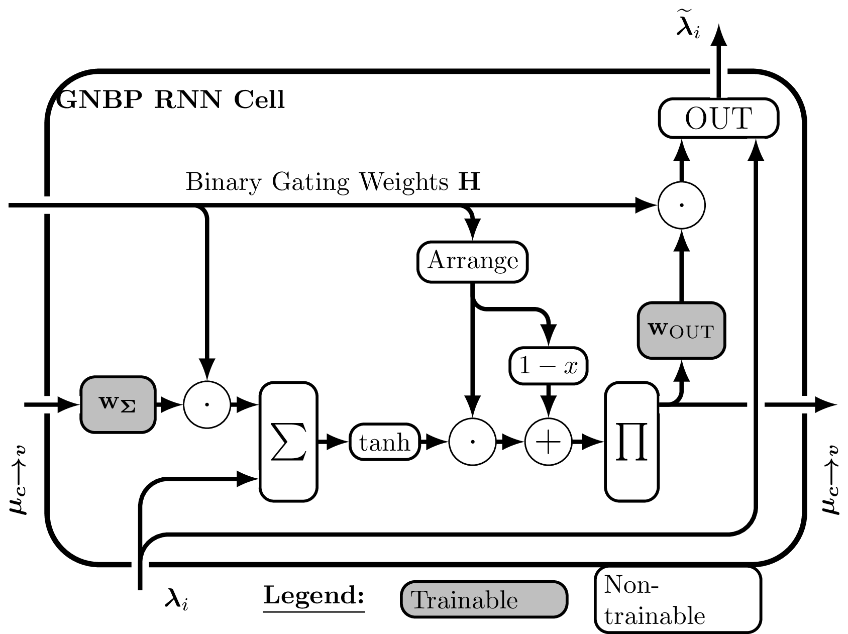
In a previous paper, a fully trainable, interpretable and low complexity version of the NBP has been proposed in the form of an RNN cell (see Fig. 2 and the original publication [11]). The main advantage of this generic model was to be able to learn to decode \((n,k)\) LBC by finding a valid PC matrix and construct the associated TG without prior knowledge of the code using gating weights. Similarly to the NBP, edges weights were used to improve the decoding performance in the presence of short cycles. To reduce the complexity, the NBP equations were simplified to: \[\mu_{v_i \xrightarrow[]{} c_j} = \lambda_i + \sum_{l \neq j}{\omega_{i,l}^{(\mu)}\mu_{c_l \xrightarrow[]{} v_i}} \label{eq:sum_GNBP}\] \[\widetilde{\lambda_i} = \lambda_i + \sum_{l}{\omega_{i,l}^{(\widetilde{\mu})}\mu_{c_l \xrightarrow[]{} v_i}} \label{eq:out_GNBP}\] This form is more compact than standard NBP as there are no weights for the inputs LLR and the message weights of equation [eq:sum_GNBP] do not depend on the destination check nodes anymore. These modifications reduce the complexity, potentially at the cost of a slight reduction in model expressiveness, although no significant performance degradation was observed w.r.t NBP. This generic architecture is a significant enabler for code exploration as will follow in this paper.
Generic Linear Block Code Neural Belief Propagation Auto-Encoder
This work focuses on the joint design of short to medium sized LBC matrices and associated weighted BP decoding structures using ML techniques. The idea is to guide the design of code matrices based on the decoder structure rather than optimizing the decoding of a potentially flawed code w.r.t. the decoder. An AE model is proposed to represent this problem.
System Model
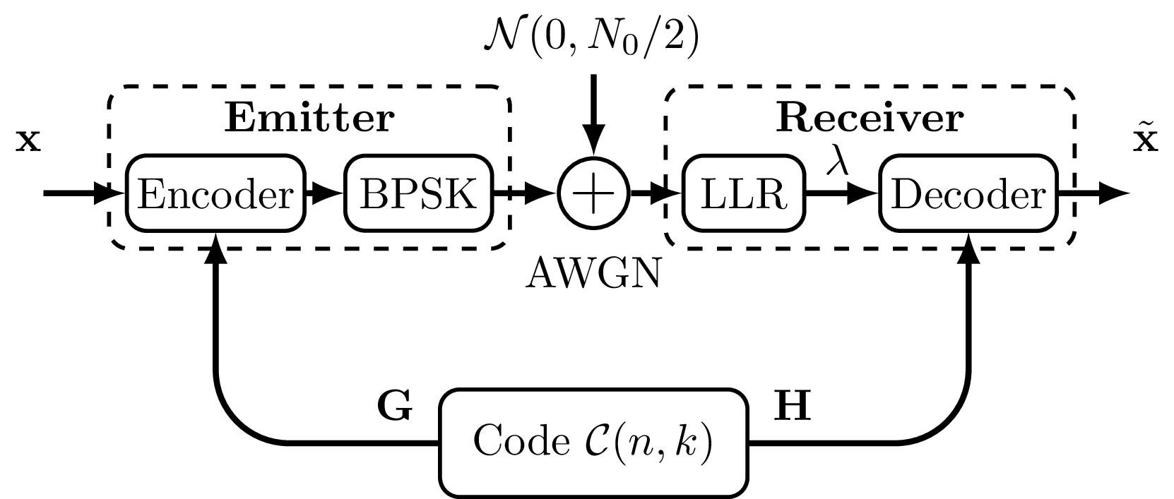
The communication scheme of Fig. 3 is considered. Inputs words are encoded based on the generator matrix \(\mathbf{G}\). A Binary Phase-Shift Keying (BPSK) modulation is applied and the symbols are sent through an Additive White Gaussian Noise (AWGN) channel with real noise power \(N_0/2\). LLRs of the received samples are decoded based on the PC matrix \(\mathbf{H}\).
The next sections describe the main identified challenges to learn short to medium size coding and decoding schemes using ML techniques and propose an AE structure to address them.
Learning to Code: Main Challenges
Differentiability of the Models
Gradient based ML techniques require the differentiability of the models to be trained. Proposed AE models in the domain of PHY layer can present several non differentiability issues related to the channel, the digital modulation, and when considering channel coding, the extensive use of finite field (e.g. \(\mathbb{F}_2\)) and associated modulo arithmetic based on eXclusive OR (XOR). The trainability of the model can also be impacted by many other optimization issues such as non-convexity, non-smoothness and non-linear separability of the loss function. Differentiable structures and approximations must be defined to circumvent such issues, thus allowing the back-propagation of gradients during the model training.
Scalability - the “Curse of Code Dimensionality”
A key factor for the adoption of AI/ML-based (de)coding methods is the scalability of the proposed models and their associated training schemes. As the number of possible words in an \((n,k)\) code is \(2^k\), even for relatively small codes it becomes impossible to use exhaustive training data-sets that include all words. It is therefore necessary to find structured architectures and learning procedures that allow the training on a subset of the possible data-words while ensuring the generalization to the remaining words during execution of the coding scheme in real operation conditions.
Linear Block Code Neural Encoder
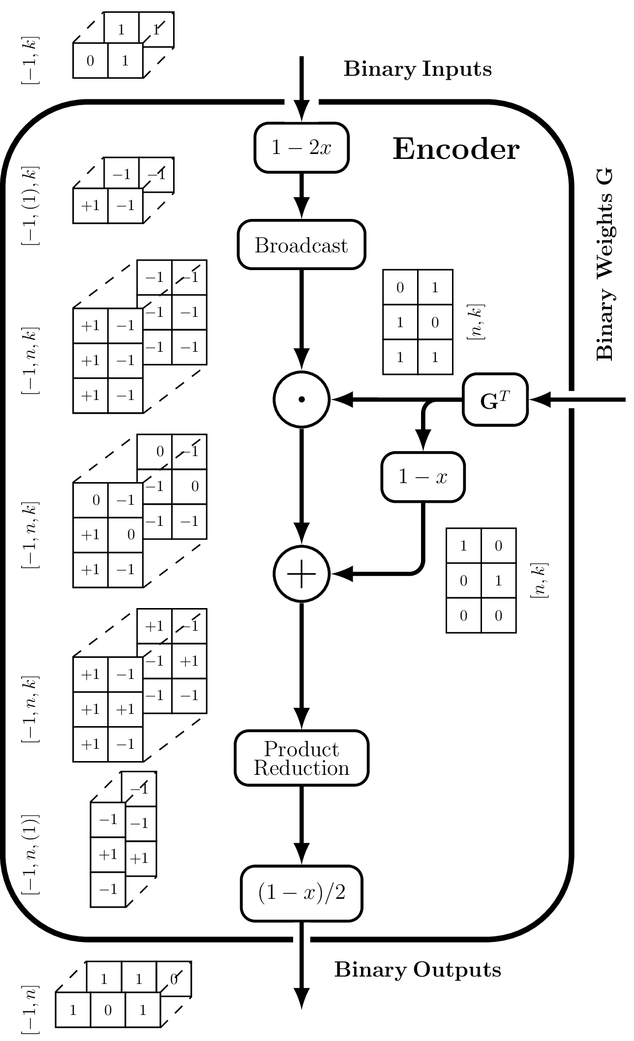
The first block of the proposed AE is the LBC encoder. The objective of this block is to encode binary words of size \(k\) into coded representation of size \(n\) based on a set of trainable parameters representing the code’s generator matrix \(\mathbf{G}\) provided, in the present work, by an external “bridge” model. The proposed encoder block describes linear combination in \(\mathbb{F}_2\) by representing the XOR function as a differentiable product of bipolar symbols (Fig. 4):
Binary words of size \(k\) are converted into bipolar form (
i.e.
\(\{0;1\}\) are mapped to \(\{+1;-1\}\)).
Inputs are broadcasted and multiplied by trainable external binary weights, i.e. the code’s generator matrix \(\mathbf{G}\), thus selecting the bits participating in each of the \(n\) encoding equations.
For the variables that were not selected the neutral element of the product (\(+1\)) is added.
Finally, a product reduction is performed for each of the \(n\) encoding equations.
The proposed architecture works if the weights \(\mathbf{G}\) and inputs are indeed binary. Since the encoder inputs are also those of the AE model, it is not difficult to guarantee this condition for the latter. However, this is more difficult in the case of the trainable weights fed to the encoder which require the loss function to remain differentiable w.r.t. them. Several solutions could be thought of, such as sigmoidal activation applied to the weights, regularization methods, sampling techniques [28], discrete functions trained using REINFORCE algorithm [29], Straight-Through Estimator [30] or a stochastic binarizer [31] as used in [20]. In this work, a differentiable approximation of the step function, inspired by the idea of differentiable bypass [32], is used. The idea is to apply a non-differentiable step function on a forward pass of the NN and approximate the gradient by a differentiable approximation of the step, a sigmoid in the present case, during the backward pass. This functional block will be referred to as a Differentiable Step Function (DSF): \[\left\{ \begin{aligned} &f(x) &=& \: \mathrm{step}(x) \\ &\frac{df(x)}{dx} &=& \: \frac{d\sigma(x)}{dx} = \sigma(x)\sigma(1-x) \\ \end{aligned} \right.\] where \(\sigma(x)\) denotes the sigmoid function.
The DSF is applied to the weights G before being used by the encoder as will be further detailed in Section 3.5.
Gated Neural Belief Propagation Decoder
The decoder is based on the GNBP RNN Cell introduced in Section 2.2.3 and inspired from a previous publication[11] although with two minor modifications:
The trainable binary gating weights defining the decoding TG architecture are now provided by an external “bridge model”. These weights represent the PC matrix of the code, \(\mathbf{H}\).
The refine gate mechanism that was used in [11] to ensure saturated sigmoid functions is now replaced by the DSF which is applied directly inside the aforementioned bridge model.
Proposed Auto-Encoder Architecture
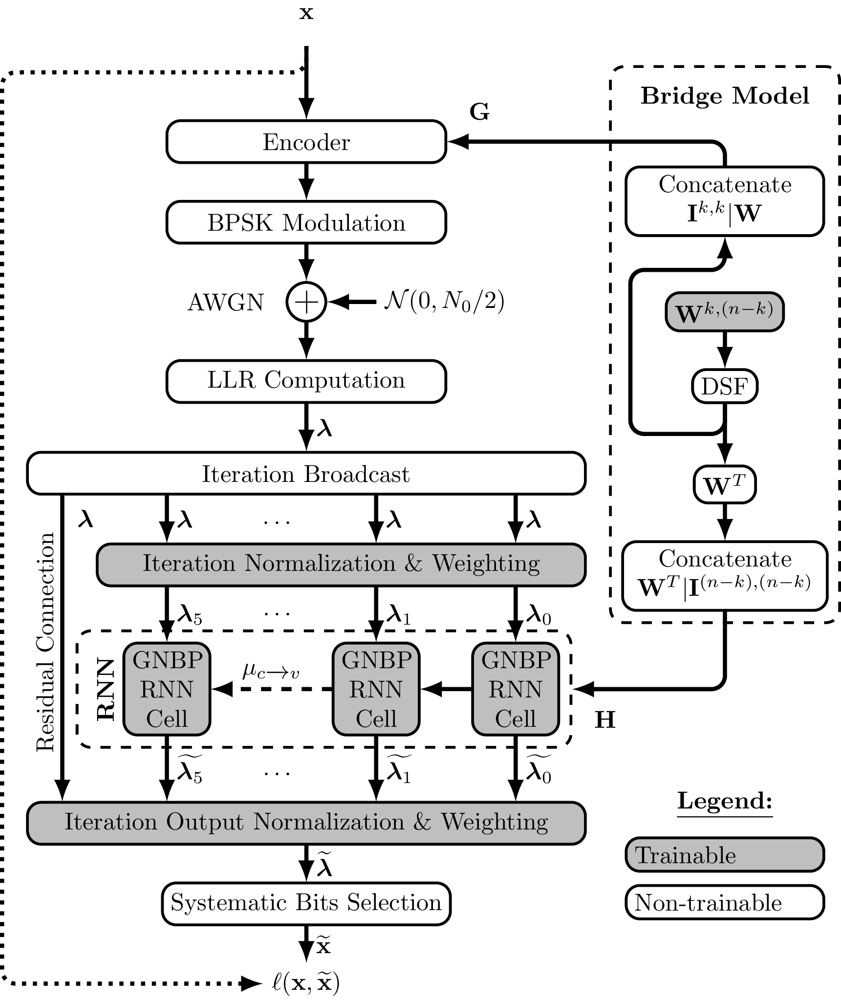
The proposed AE architecture for the joint design of a LBC and associated GNBP decoder consists of the proposed encoder and decoder models at the transmitter and receiver sides (Fig. 5). The encoder weights and corresponding decoder gating weights that represent the code matrices are provided by a third “bridge model” to ensure that they are continuously matched. The use of such a weight sharing procedure makes the training easier and thus reduces training time. A simple way to implement this procedure is to restrict the learned code to generator and parity-check matrices in standard forms. It enables a direct and differentiable conversion between \(\mathbf{G}\) and \(\mathbf{H}\), as described in Section 2.1. The standard form offers the advantage of a reduced number of trainable code parameters. In addition, it reduces the complexity of the encoding and possibly avoids costly decoding in the absence of errors, e.g. by computing a Cyclic Redundancy Check (CRC) of the complete data-frame before checking the syndromes of it’s constituent code-words and eventually initiating decoding procedures. However, the standard form can be detrimental to the performance of a BP-based decoder as it generally leads to denser PC matrices. How to circumvent this problem is left for future work.
Input words are encoded, according to the trainable matrix \(\mathbf{G}\) provided by the bridge model, using the encoder introduced in Section 3.3. The resulting code-words are modulated using a BPSK and sent over an AWGN channel. On reception, the LLR of the code-words are computed and normalized by their per-codeword mean absolute value. The normalized LLR are broadcasted and weighted on a per-iteration basis and provided to the GNBP RNN decoder as follows: \[\boldsymbol{\lambda_i} = w_i^{(\mathrm{in})}\frac{n\boldsymbol{\lambda}}{\sum_{j=1}^n |\lambda_j|} \quad \forall i \in \{1,...,n_\mathrm{iter.}\}\] After GNBP decoding based on the trainable matrix \(\mathbf{H}\) provided by the bridge model, the iterations results and the residual connection are normalized and weighted for recombination as follows: \[\widetilde{\boldsymbol{\lambda}} = w^{(\mathrm{residual})}\frac{n\boldsymbol{\lambda}}{\sum_{j=1}^n |\lambda_j|} + \sum_{i=1}^{n_\mathrm{iter.}}w_i^{(\mathrm{out})}\frac{n\widetilde{\boldsymbol{\lambda}_i}}{\sum_{j=1}^n |\widetilde{\lambda_{i}}_j|}\] The systematic bits are selected as the first \(k\) LLR of the decoded code-words and are fed to a sigmoid function to assign them binary-like values. In an AE learning scheme, the inputs are identical to the associated labels. Hence, the loss function is computed as the Binary Cross-Entropy (BCE) between the input and decoded binary words: \[\ell(\mathbf{x},\mathbf{\tilde{x}}) = \mathrm{BCE}(\mathbf{x},\mathbf{\tilde{x}}) = \mathrm{BCE}\left(\mathbf{x},\sigma(-\widetilde{\boldsymbol{\lambda}})[0:k]\right)\] Unless otherwise specified, the RNN decoder is configured to execute the equivalent of 5 BP iterations. The use of a residual connection bypassing the decoder and the iterations results recombination mechanism are design choices deemed to facilitate gradient back-propagation during training. The total number of trainable parameters of the proposed architecture is defined as follows: \[n_{\mathrm{param.}} = \underbrace{k(n-k)}_{\text{Systematic code}} + \underbrace{2n(n-k) + 2n_{\mathrm{iter.}} + 1}_{\text{GNBP decoder}}\]
The use of shared parameters and a structured architecture allow for a controlled number of trainable parameters (Tab. 1). Furthermore, for a fixed code-rate, the number of parameters of the AE evolves in \(\mathcal{O}(n^2)\) ensuring the scalability of the proposed architecture on that matter, at least in the short-to-medium block size regime of interest to the present study. Thanks to the definition of matched \(\mathbf{G}\) and \(\mathbf{H}\) matrices in standard form, the bridge model ensures an efficient training phase. The interpretable structure of the model allows the learned code to be extracted and used with other LBC decoding schemes, possibly within legacy, non-AI based systems. The enhanced weighted decoding procedure based on the RNN GNBP cell is jointly trained with the coding scheme. In conclusion, the proposed differentiable AE architecture allows the efficient training of performing LBC suitable for a BP-based decoding.
| \(n\) | \(k\) | \(n_\mathrm{param.}\) |
|---|---|---|
| 128 | 64 | 20491 |
| 63 | 36 | 4385 |
| 45 | 3089 | |
| 31 | 11 | 1471 |
| 16 | 1181 | |
| 8 | 4 | 91 |
Data-sets, Training & and Evaluation Procedures
In a naive approach, learning a code of size \((n,k)\) would require to use a training data-set including all the \(2^k\) words. This number grows exponentially with the code size and can become prohibitively large. In the case of LBC and under symmetric assumption on the channel and the decoder (implying in the case of NN based decoders the use of symmetric activations, absence of biased units, etc.), it is common to train or evaluate a decoder only with the zero code-word while guaranteeing performance on the complete code [23]. Nevertheless, the training of the encoder is also considered in this work, thus requiring the use of different words. The proposed encoder ensures that all code-words are linear combinations of the basis of the vector subspace of the code. Hence, the model can be trained using only the basis vectors of the words thus reducing the training data-set size from an exhaustive data-set of \(2^k\) words to only \(k\) words.
It should also be noted that since the XOR function used in the encoder is a non-linearly separable operator, optimizing the weights upstream this function can be challenging for a high input cardinality. Indeed, the non-linear separability of the operator prevents from identifying the individual contributions of each input in the final results as for a linearly separable operator such as the sum. Still, one way to ensure that the individual contributions are identifiable in the final results is to ensure that there is only one non-zero input contributing to the XOR in each dataset entry e.g. by considering only standard basis vectors as inputs, hence the adopted data-set. Similarly, the decoder uses product operators, particularly challenging w.r.t. the optimization of the model for similar reasons. Following the same intuition as before, one should carefully choose the channel noise level ensuring a controlled amount of bit flips per code-word. Gaussian noise sampled by the NN model with a fixed \(E_b/N_0\) of 4 dB has shown empirically to provide good results.
The model is trained with RMSProp optimizer [33] using batch-size of 64 words and 25 steps per epochs until an early stopping criterion is met (200 epochs without improvement) or the maximum number of epochs, set to 1 000, is reached (a significant margin is used as it has been experimentally observed that the AE usually converges to its best level of performance within the first 100 epochs). The Learning Rate (LR) is initially set at \(10^{-1}\) and follows a decaying schedule on plateau: when the model does not improve for 50 epochs the LR is reduced by 20%. The validation data-set is randomly sampled from the \(2^k\) possible words in batches of size 64 which are used to monitor the model progress on the real encoding/decoding task, i.e. transmitting and recovering any of the possible words with as few errors as possible. A BCE loss function, particularly suited for binary error evaluation, is used. The model weights representing the code, \(\mathbf{W}\), are initialized uniformly at random on the \([-0.01;+0.01]\) range. The GNBP decoder weights are initialized at ’1’. After training, the model is evaluated on randomly sampled words from the \(2^k\) possible words with \(E_b/N_0\) ranging from 0 dB to 6 dB. To ensure a reliable Bit Error Rate (BER) evaluation at each \(E_b/N_0\) level, new words are sampled and provided to the model until the 95% confidence interval, computed using Agresti-Coul method [34], on the estimated model BER performance is within the estimated BER +/-5% interval, i.e. there is a 95% probability that the true value of the BER lies in-between +/- 5% of the estimated BER2.
Results
The following sections describe the results obtained with the proposed model in various experiments. At first, (8,4) codes will be used to illustrate the approach and to formulate hypotheses as to why it is likely to produce successful results. A second experiment will study in depth the training of the AE on a (31,16) code size and compare its performance with those of a standard BCH code in standard and non-standard forms. The observed performance gain will be investigated in a short ablation study on a (31,11) code size. Scalability of the approach will then be evaluated on (63,36) and (63,45) code sizes and compared to some existing results, notably with the NBP approach [4]. In addition, a comparison of the complexity of the different decoders will be proposed. Finally, the approach will be tested against other state-of-the-art codes with sizes up to 128 bits, including LDPC codes better suited for BP decoding than BCH codes.
(8,4) Code: Illustration of the Proposed Concept
The model is first tested on a (8,4) code size and compared with a classic hand-crafted code: Extended Hamming (8,4) (Fig. 6). The performance of the AE model ([plot:84AEGNBP]) is compared to those of MLD3 ([plot:84HMLD]) and BP ([plot:84HBP]) decoders applied to the Hamming code. MLD is also applied, after training, on the code matrix designed by the AE ([plot:84AEMLD]). This allows to evaluate the proposed code’s raw algebraic performance independently of the decoder target.
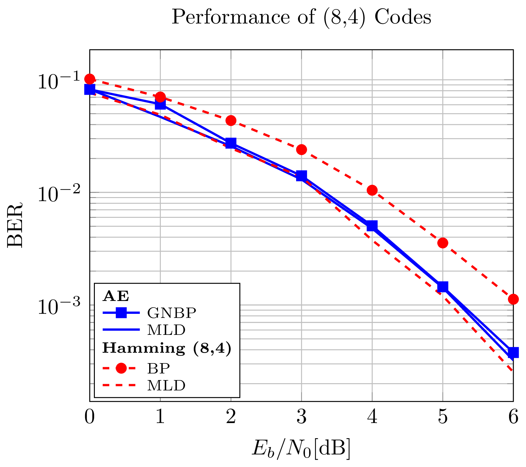
As demonstrated by the MLD performance curves, the learned code is not as good as the Hamming code in terms of algebraic properties. Nonetheless, the proposed AE outperforms, by a significant margin, a standard BP decoder applied to Hamming code. Fig. 7 represents the PC matrices as well as the corresponding TG for both Hamming code and the best AE designed code out of 5 trials. Several interesting algebraic properties are to be noted when comparing both codes. As one can see the learned coding scheme is an irregular coding scheme.
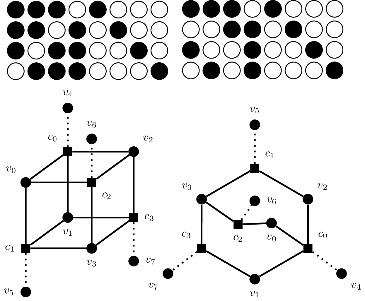
The minimum distance of the learned code is equal to 3 while the minimum distance of the Hamming (8,4) code is equal to 4. This explains why the proposed coding scheme is less efficient in terms of MLD performance. Still, the average Hamming distance is of 4.26 for both codes. As one can see, while the density of the PC matrix is reduced, the girth of the TG is augmented in the case of the learned code. Indeed, the Hamming code presents a density of \(\delta = 16/32 = 0.500\) and a girth of 4 with 6 associated cycles, whereas the learned code has a density \(\delta = 13/32 = 0.406\) and a girth of 6 with 3 associated cycles. These properties are key in the performance of a BP decoder and can explain the performance gain of the proposed code when associated to a GNBP decoder.
These results are a good illustration of the proposed concept: instead of trying to find a code with good properties such as minimum distance, the model proposes a code that improves the performance w.r.t. the targeted BP-like decoder. In the case of such a short code, it is worth noting that even a naive MLD is not complex and is eventually more efficient than 5 iterations of a BP-like approach. However, this statement quickly becomes untrue as the code size increases.
(31,16) Codes: Statistical Study of Model Training
Model Performance During Training
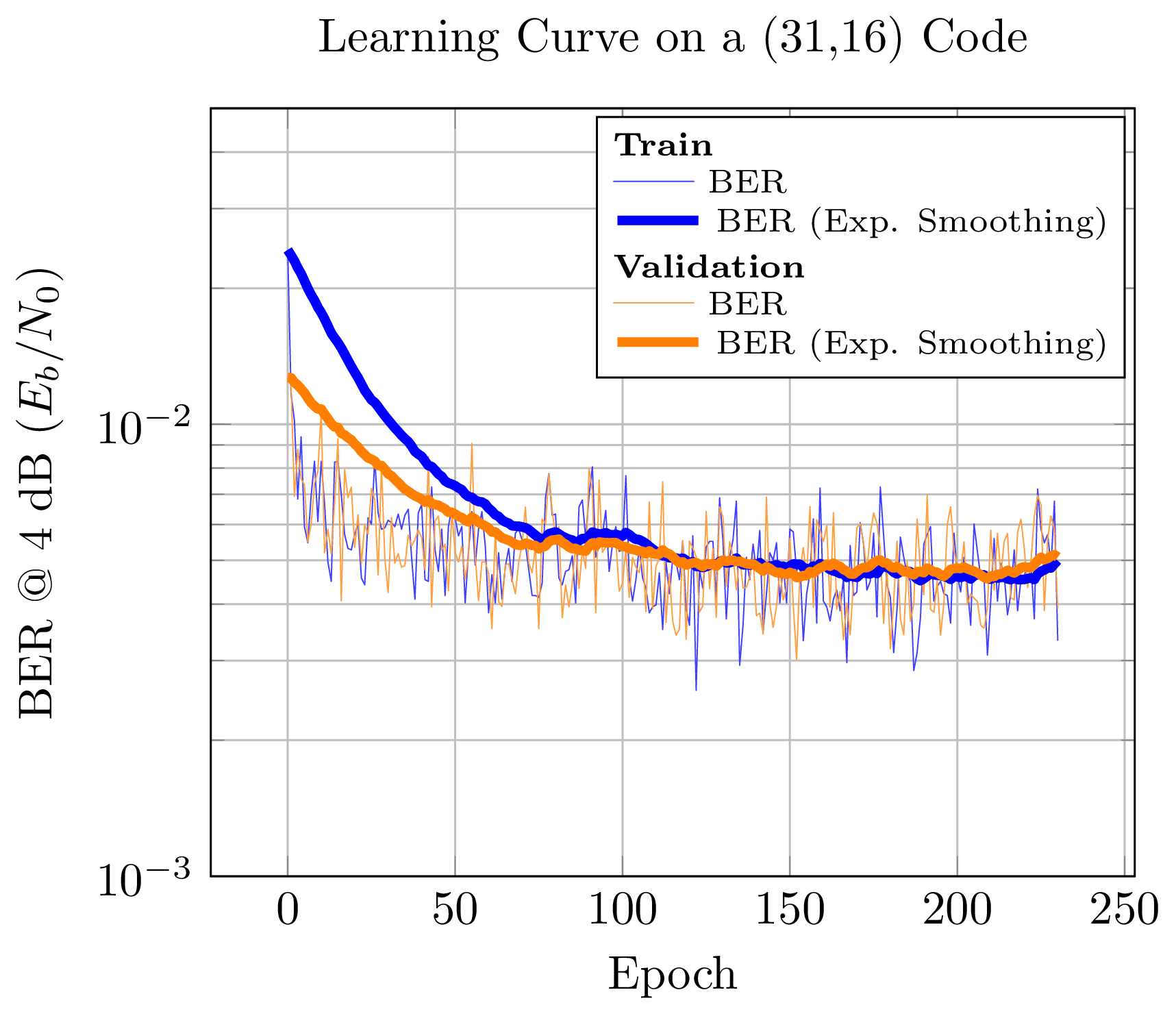
The proposed model’s BER metric is measured during training to assess the existence of a learning process on a (31,16) code. Fig. 8 shows the BER at the selected training \(E_b/N_o\) of 4dB evaluated at each epoch for the training ([plot:3116Train]) and validation ([plot:3116Val]) data-sets. Although noisy, these curves show a clear decrease in BER during training as supported by the corresponding smoothed metrics ([plot:3116TrainSmoothed] / [plot:3116ValSmoothed]). During training the BER is roughly divided by a factor 10, from \(\approx 2.5 \times 10^{-2}\) to a minimum of \(\approx 2.5 \times 10^{-3}\).
Training Repeatability
The design of an AI/ML-based error correction scheme can usually be performed offline and only the best learned coding scheme selected for implementation in the final communication system. Nevertheless, it is interesting to study the performance consistency of the learned codes as an empirical assessment of the model training reliability. Furthermore, in future work, such model could be integrated into E2E communication systems relying on the joint learning of equalization, (de)modulation and (de)coding, etc. Such scenario would require an efficient and reliable online learning process.
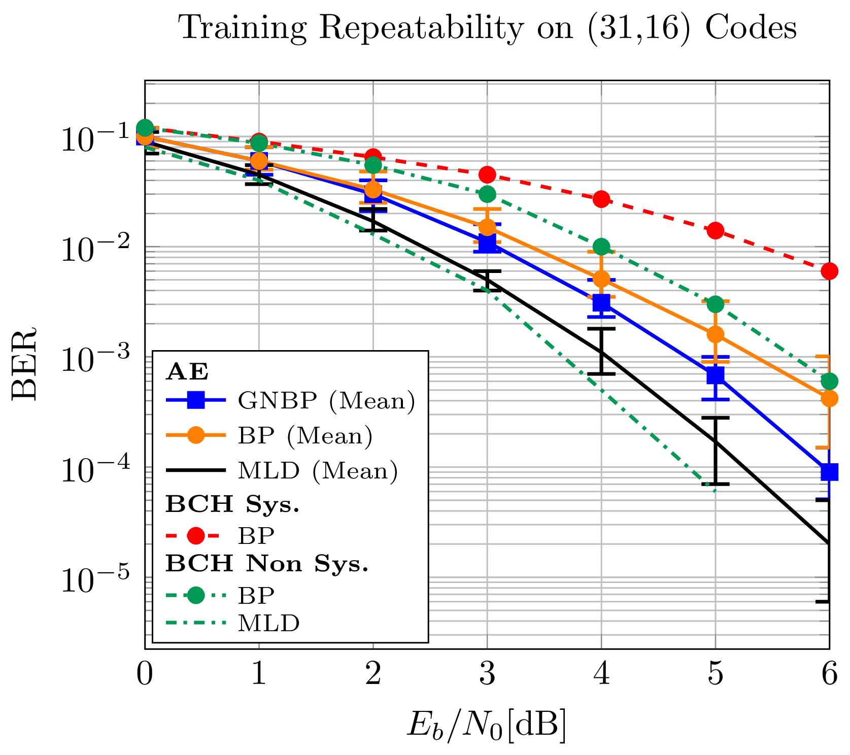
The min-max interval of BER performance of the proposed AE ([plot:3116AEGNBP]) across 50 independent trainings (Fig. 9) demonstrates the model’s ability to learn a larger code size of (31,16) and shows a reliable and repeatable training process with relatively small variations between runs. Indeed, Fig. 9 shows approximately 0.5 dB between the worst and best model in the asymptotic regime. The repeatability of model training being demonstrated, the following results of this paper will present only the best training out of 5 trials as an estimate of the achievable performance of the AE and thus reduce the effective simulation time.
Additionally, Fig. 9 shows the performance of a non-systematic BCH code (31,16) from the literature [35], evaluated on MLD ([plot:3116BCHNSYSMLD]) and BP ([plot:3116BCHNSYSBP]) decoders. A systematic version of the BCH code obtained by the Gauss-Jordan elimination method is also evaluated with a BP decoder ([plot:3116BCHSYSBP]). Finally, the code learned by the AE is extracted and evaluated on these same MLD ([plot:3116AEMLD]) and BP ([plot:3116AEBP]) decoders. Similarly to what has been observed previously with the extended Hamming code, the learned (31,16) code has slightly worse MLD performance than the BCH code (yet almost equivalent in the case of the best model) but is significantly more competitive when using the BP or GNBP decoders compared to the standard BP decoder applied to both systematic and non-systematic BCH codes. It can also be noted that a systematic form is generally detrimental to the performance of a BP decoder. Indeed, it artificially increases the density of the PC matrix in its redundant part which in turn can reduce the girth of the code.
Correlation Between Decoders Types and their Performances
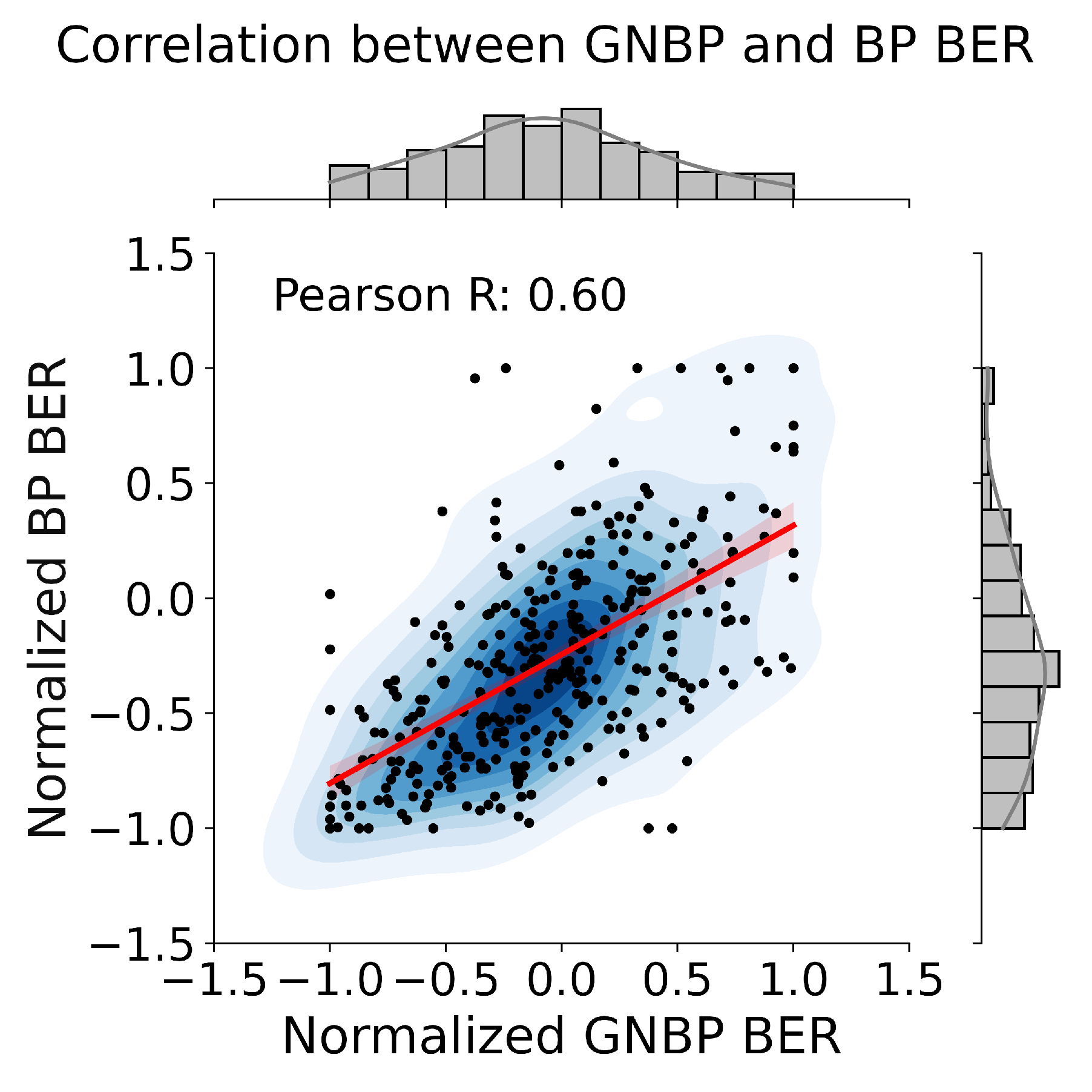
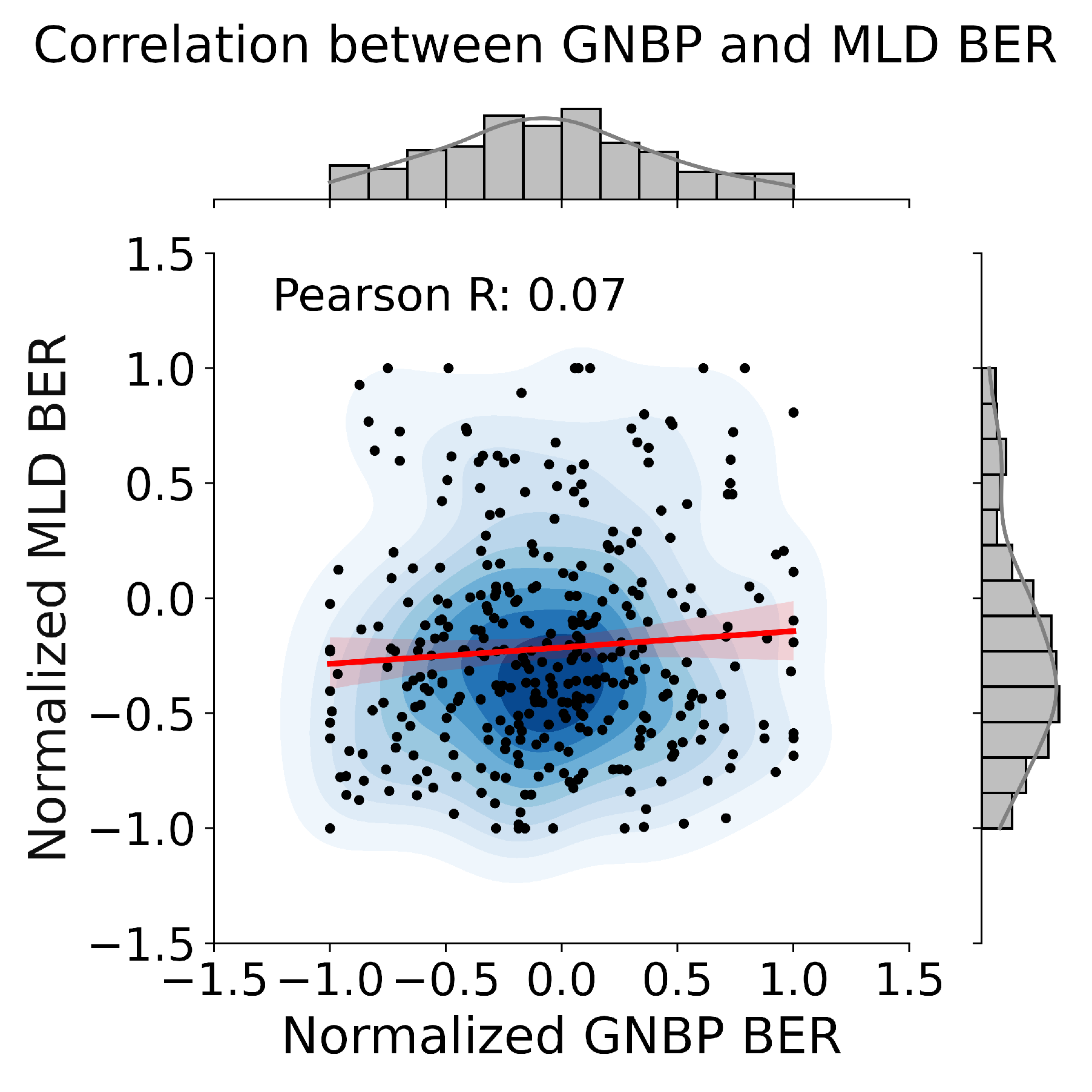
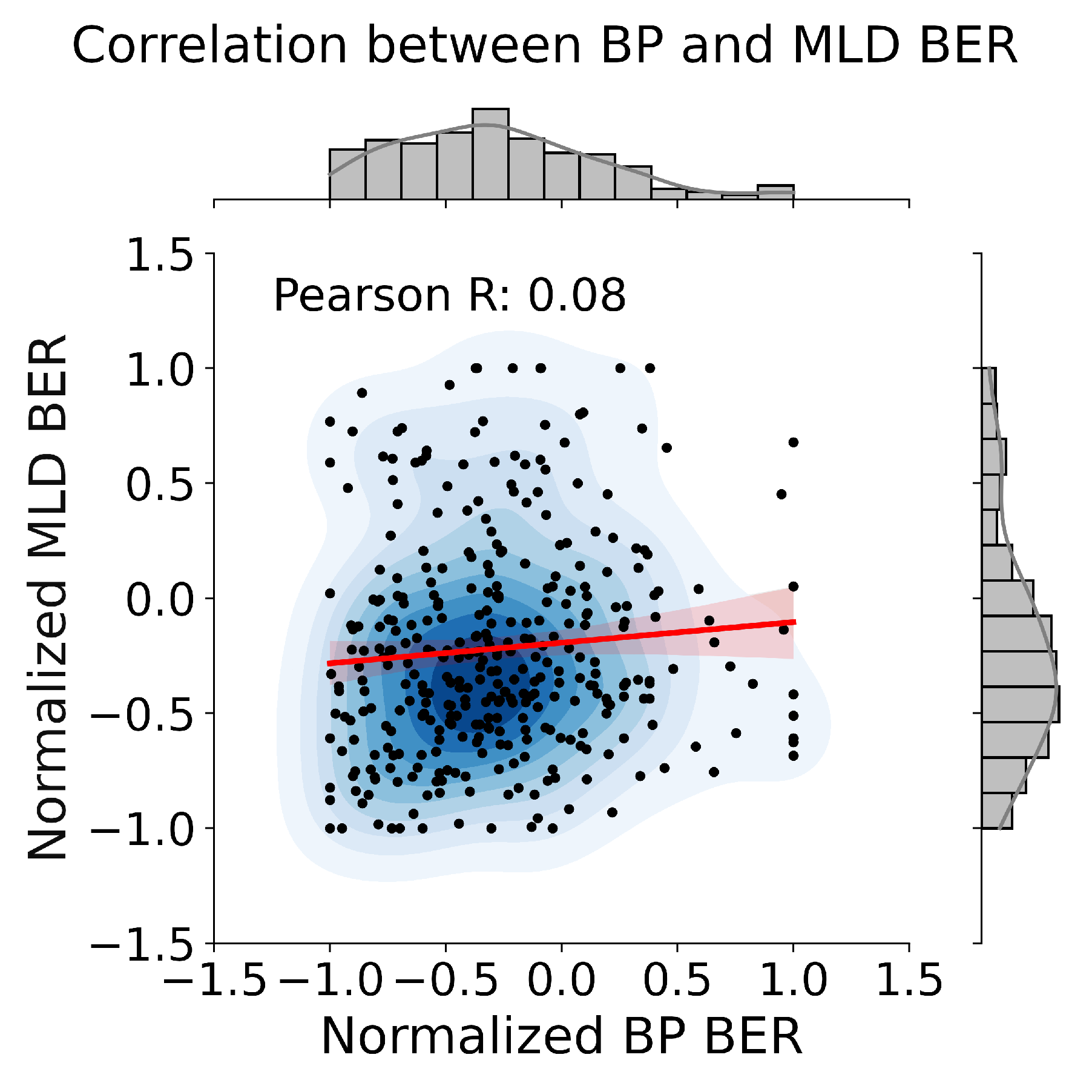
Fig. 9 showed the span of the BER performance of the 50 learned codes with different decoders. One question is whether good code performance with one decoder type is generally associated with good performance with the other decoders. To answer this question, the performance correlations of a given learned code between GNBP and BP (Fig. [fig:GNBP_vs_BP_corr]) or MLD decoders (Fig. [fig:GNBP_vs_ML_corr]) and between BP and MLD decoders (Fig. 10) are provided. For each decoder and \(E_b/N_0\), the BER performance of the 50 learned codes are normalized on the \([-1;+1]\) range and aggregated on a single plot. As one can see, the performance of the learned code evaluated on BP decoder are correlated with their performance on the GNBP decoder. This was foreseeable since the GNBP decoder is derived from the BP decoder. On the contrary, the performance of the learned code evaluated on the GNBP or BP decoders are not correlated with those of the corresponding MLD decoder.
Degree Distributions of Learned Codes
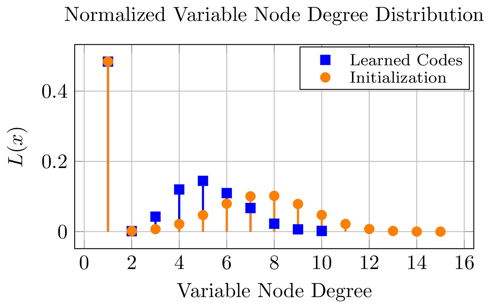
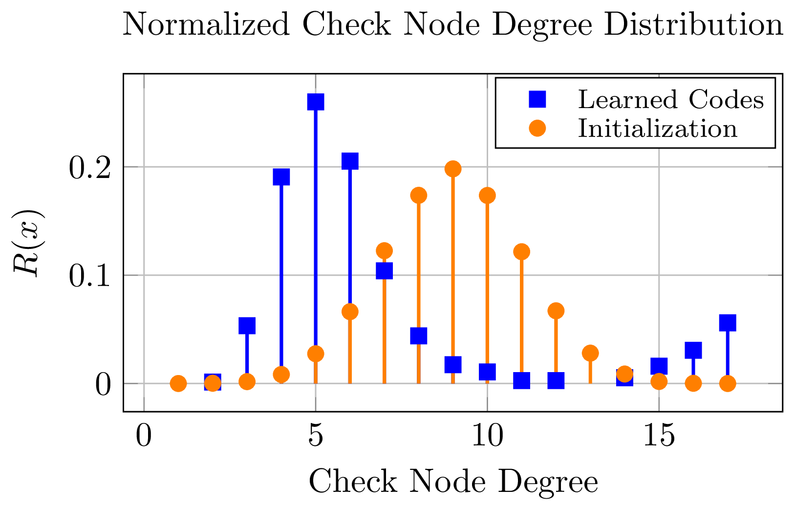
In an attempt to explain the observed performance from a code design perspective, and even though only small codes are considered here, the normalized variable and check node degree distributions are computed for each of the 50 learned PC matrices and averaged over all the trainings (Fig. [fig:average_var_degree_distribution_31_16] and 11). These distributions ([plot:VarDegree]) are compared with those at model initialization ([plot:VarDegreeInit]). In addition to demonstrating consistent results across trainings and showing that the learning procedure does indeed have an impact on the choice of specific, non-random structures, the learned matrices exhibit unexpected check node degree distributions. The learning procedure seems to encourage overall lower density of the matrices, which was something to be expected given the targeted BP decoder structure. On the other hand, it also seems to promote the definition of a few high degree check nodes. This behavior is not yet explained but is of interest for future studies.
(31,11) Codes: Auto-encoder Training Procedure and Ablation Study
Several questions arise from observations of previous section. What is the origin of the AE performance gain? Is it due mainly to the use of a weighted decoding procedure such as GNBP, the design of a more efficient coding scheme or a combination of both? Is it preferable to first train the coding scheme and then adapt the GNBP decoder to proposed code or learn jointly both codes and decoders as it was done in previous sections? To try to answer these questions, the AE is applied to a (31,11) code and compared to a BCH code from [35]. The influence of the different elements of the AE and their training schedules is studied to better understand the origin of the performance gain. Different schemes are compared (Fig. 12):
The full AE model as described in 3.5 to study the influence of both the learned code and the GNBP decoding scheme ([plot:3111AEGNBP]).
The code learned by the aforementioned AE model evaluated on a standard BP decoder to study the influence of the sole learned code ([plot:3111AEGNBPBP]).
A slightly different AE trained with a differentiable standard BP decoder i.e. without any GNBP decoder weights, inputs LLR weightings, residual connection or weighted outputs sum (only the result of the last iteration is selected as in standard BP decoders). This scheme is referred as “AE BP” on the Fig. 12 ([plot:3111AEBP]).
The code learned by this AE BP model used to train a GNBP decoder to study the impact of the training schedule ([plot:3111AEBPGNBP]).
The MLD performance of the codes learned by both AE (GNBP) ([plot:3111AEGNBPMLD]) and AE BP ([plot:3111AEBPMLD]) models.
A reference BCH (31,11) code [35] in both systematic and non-systematic forms evaluated with MLD ([plot:3111BCHNSYSGNMLD]), standard BP ([plot:3111BCHNSYSBP] / [plot:3111BCHSYSBP]) and trainable GNBP decoders ([plot:3111BCHNSYSGNBP] / [plot:3111BCHSYSGNBP]).
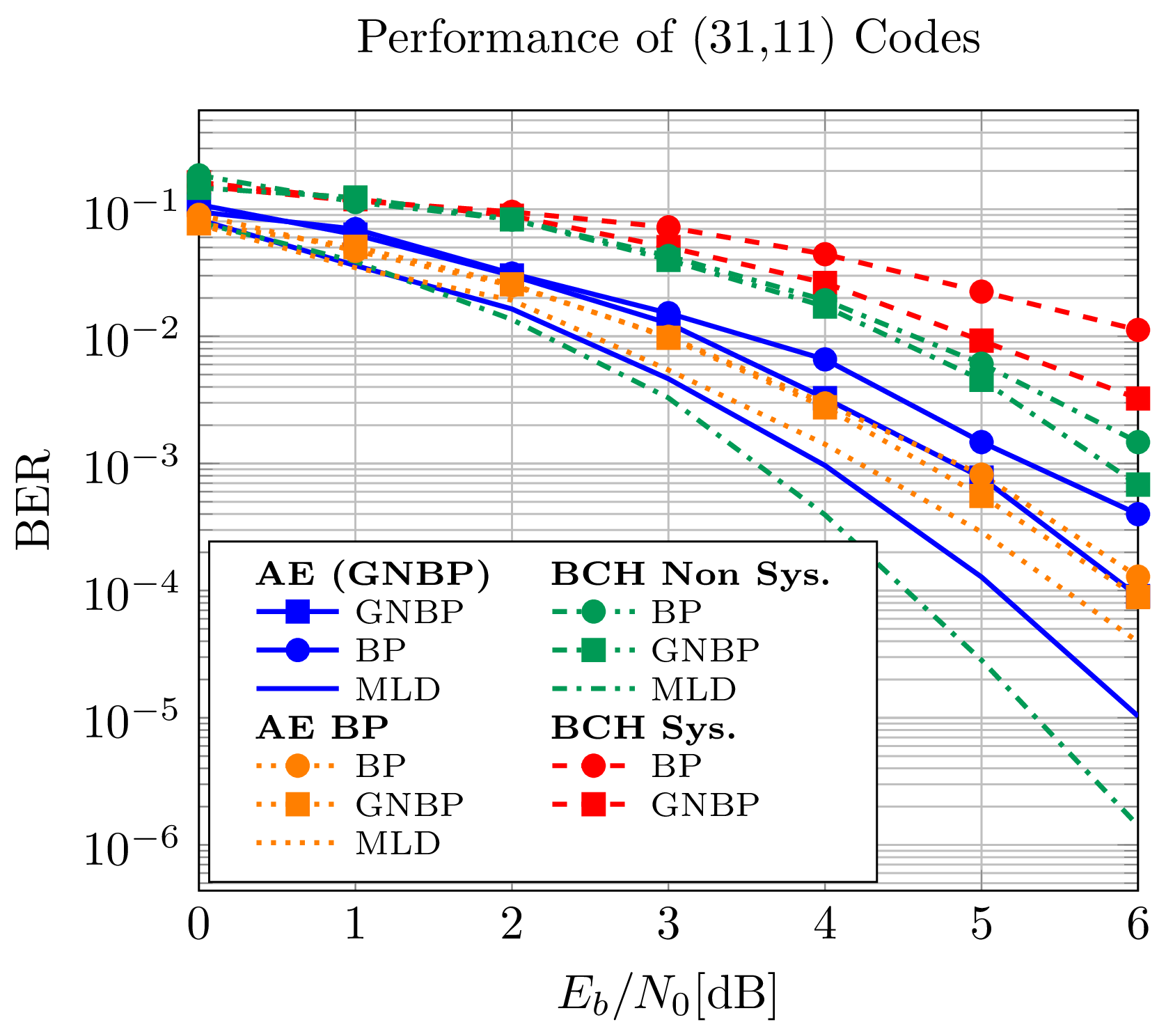
Even though a different code rate is considered, similar statements can be made on the performance of the (31,11) code to that of the (31,16) code: the MLD performance of the BCH (31,11) code is better than that of the learned coding schemes. Yet, all the proposed coding scheme outperforms by a significant margin the standard BP decoder applied to both systematic and non-systematic BCH (31,11) codes.
It appears that the design of an effective coding scheme and the use of a weighted GNBP decoding procedure can both contribute to the final performance of the AE. However, the training schedule has an impact on their relative contributions to the final performance (Fig. 12). Indeed, after learning both the code and the GNBP decoder weights, regardless of the training schedule of the different blocks involved, the AE achieves similar performance. Yet, the code learned directly with a BP decoder achieves better performance than the code learned with a GNBP decoder and subsequently evaluated on a BP decoder. Therefore, if the final goal is to run a GNBP decoder, it is more interesting to train the model directly with such a decoder rather than first training the code on a BP decoder and then learn the GNBP weights, which would take twice as much training time for a similar outcome. On the contrary, if the aim is to use a standard BP decoder, it is more interesting to train the model with such a decoder from the beginning, as this may lead to better overall results compared to a code learned on a GNBP decoder and then evaluated on a BP decoder. It is also worth noting that the performance of the AE model trained and evaluated only on a BP decoder is close to that of the AE model using a GNBP decoder. This suggests that when the coding scheme is well constructed and suffers from few defects w.r.t. a BP decoder, e.g. a small number of short cycles, the benefit of a weighted decoding procedure such as GNBP might be reduced and a simpler BP decoder could be sufficient. Nevertheless, as shown by the GNBP performance curve of the BCH code, the use of a weighted decoder can bring a significant performance gain for codes that exhibit defects w.r.t. the targeted BP decoding procedure, e.g. BCH codes, confirming results from previous works [4],[11]. However, the observed performance gain is not up to the level of the AE joint code and decoder design.
(63,36) & (63,45) Codes: Scalability and Algorithmic Complexity
Scalability to (63,36) & (63,45) Codes
To illustrate the flexibility and scalability of the proposed approach, the AE model is evaluated on higher sizes (63,36) and (63,45) codes. With such sizes the code-books include too many code-words to be included in an exhaustive data-set (Tab. 2). Additionally, the trainable part of the systematic matrices include many configurations of ’0’ and ’1’.
| Code | \((n,k)\) | \((63,36)\) | \((63,45)\) |
|---|---|---|---|
| # Code-words | \(2^k\) | \(\approx 10^{10}\) | \(\approx 10^{13}\) |
| # Basis code-words | \(k\) | \(36\) | \(45\) |
| # Different sys. PC matrices | \(2^{k(n-k)}\) | \(\approx 10^{292}\) | \(\approx 10^{243}\) |
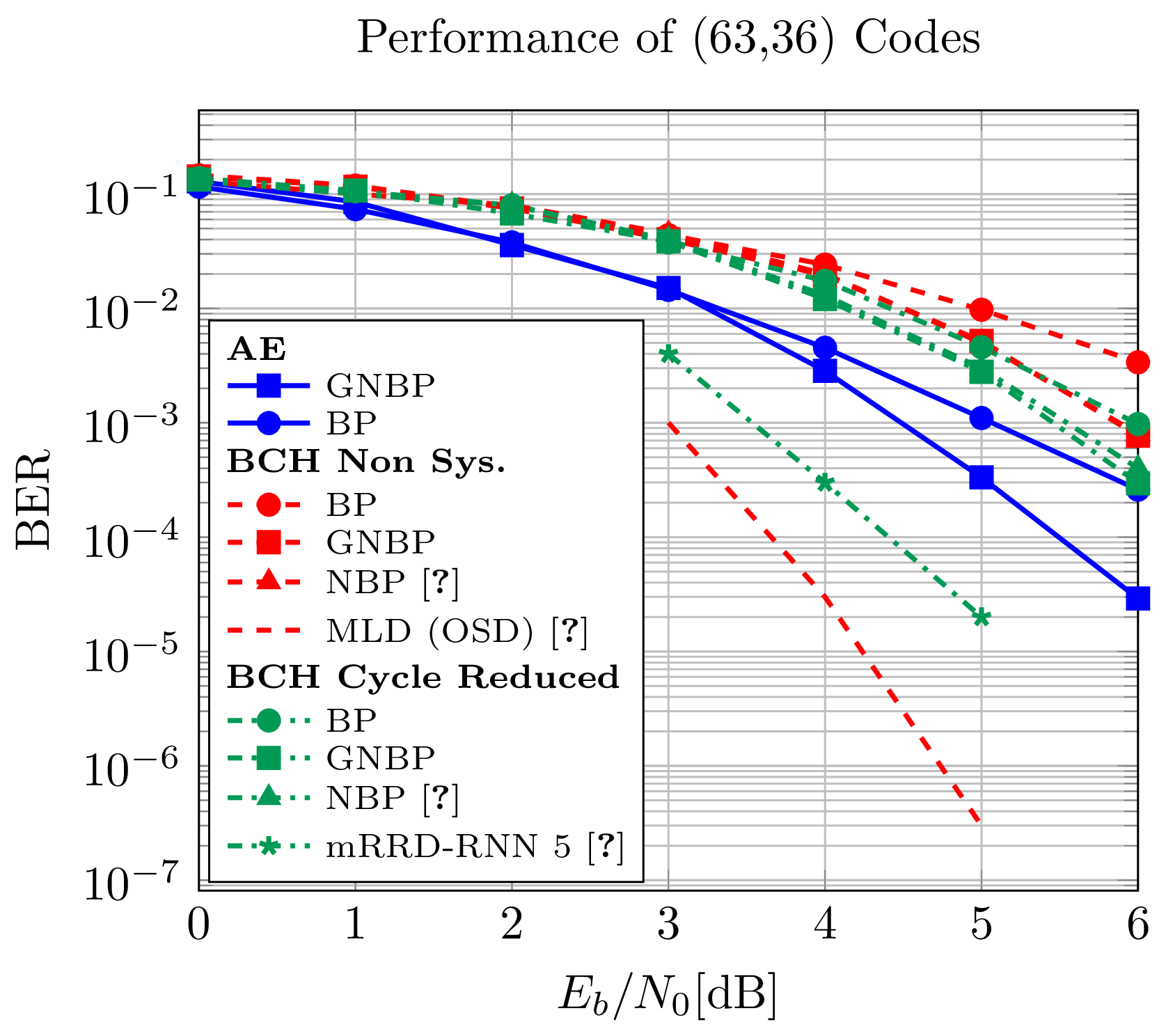
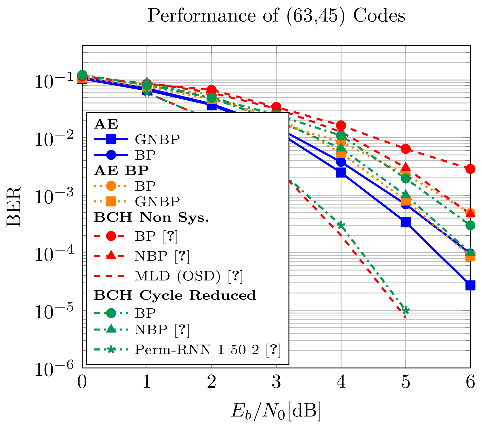
The performance of the AE ([plot:6336AEGNBP]) is compared to that of the BP ([plot:6336BCHCRBP] / [plot:6336BCHNSYSBP]), NBP ([plot:6336BCHCRNBP] / [plot:6336BCHNSYSNBP]) and MLD ([plot:6336BCHNSYSMLDOSD]) (Ordered Statistics Decoder (OSD) [36]) decoders applied to the (63,36) and the (63,45) BCH codes as described in the original Nachmani et al. publication [4]. AE BP scheme results, evaluated with both BP ([plot:6345AEBP]) and GNBP ([plot:6345AEBPGNBP]), are also provided for the \((63,45)\) code. In contrast to Section 5.3, this scheme is here not on par with the AE GNBP. The performance of mRRD-RNN ([plot:6336BCHCRmRRDRNN]) and Perm-RNN ([plot:6345BCHCRPermRNN]) parallel BP decoders from [4], [27] are also provided as examples of close to MLD decoders, although at a much higher complexity (Fig. [fig:63_36_BER] and 13). In addition, the GNBP decoder is applied on BCH (63,36) codes ([plot:6336BCHCRGNBP] / [plot:6336BCHNSYSGNBP]), demonstrating similar performance to that of the NBP. For both sizes, the AE outperforms BP and NBP decoders with different BCH PC matrices forms. Even the code learned by the AE evaluated with a BP decoder ([plot:6336AEGNBPBP]) outperforms GNBP decoder applied on the BCH codes, at least in the considered \(E_b/N_0\) regime. Again, these curves show that the design of a code tailored to the decoder provides substantial performance gain at no significant complexity cost.
Complexity Study
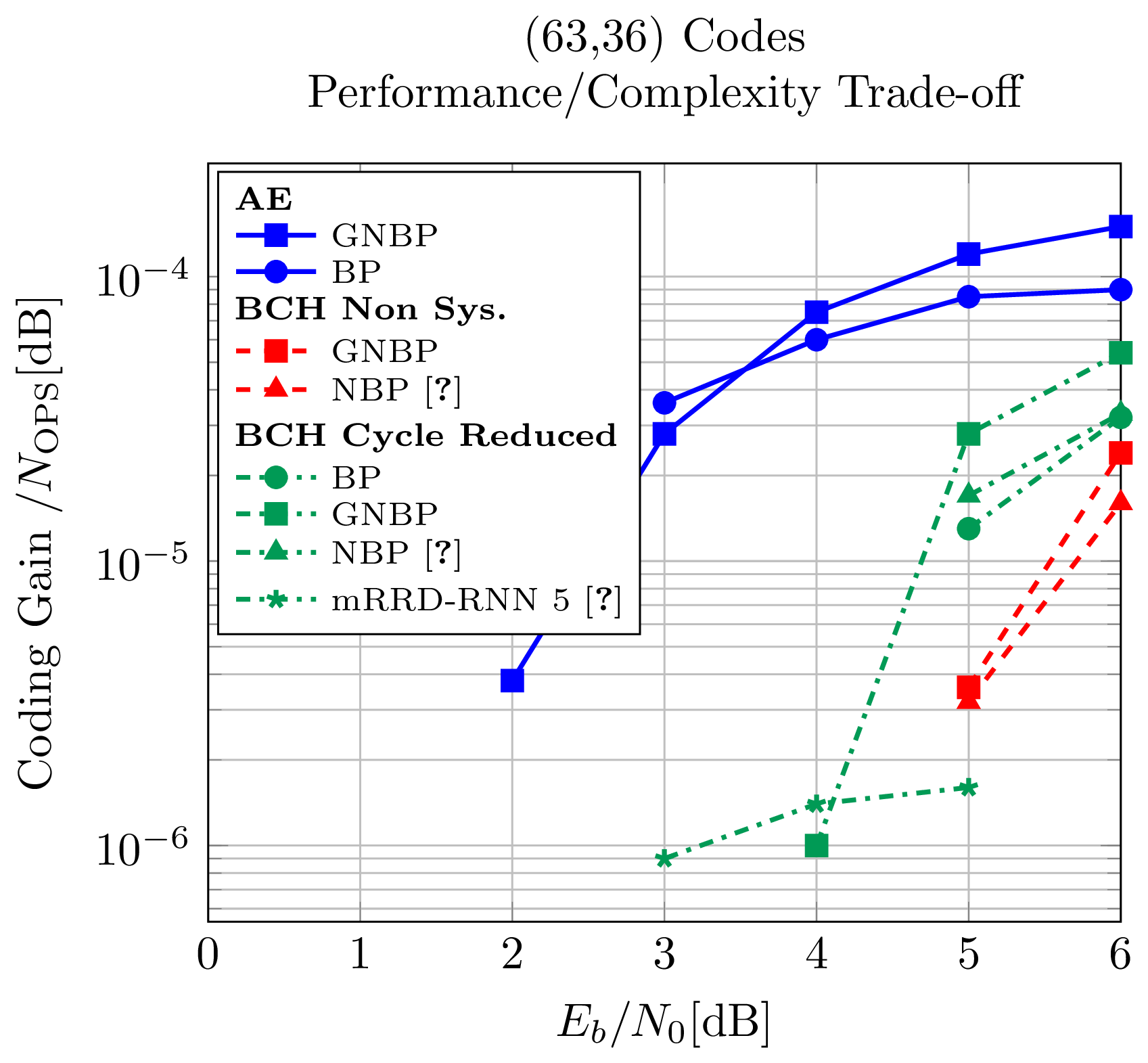
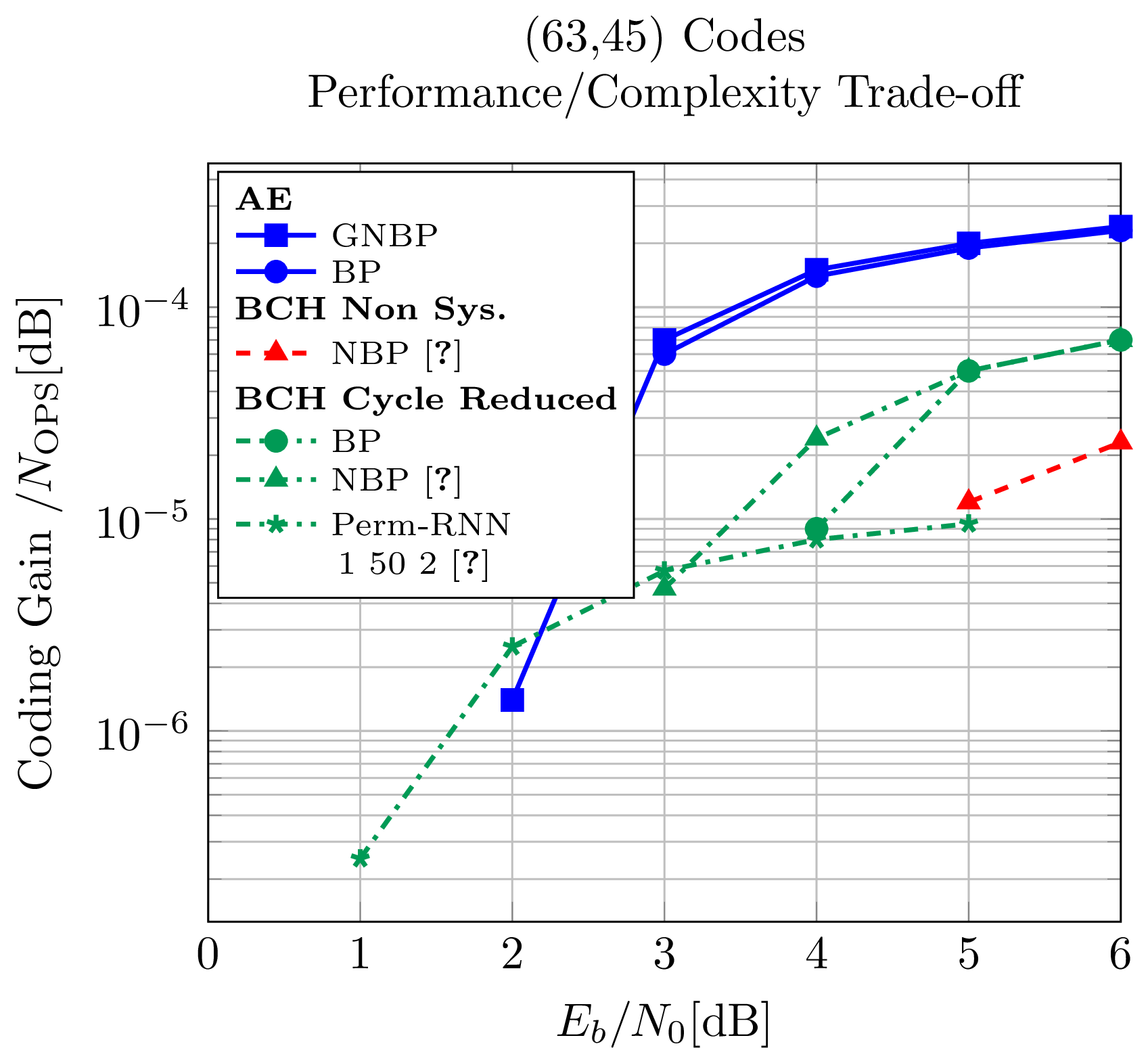
To further illustrate the advantageous performance to complexity ratio of the proposed approach, the number of decoding operations is computed for the different codes and associated decoders, as summarized in Tab. 3. The coding gain (dB) w.r.t. an uncoded BPSK is then computed for each code and decoder and normalized by the number of operations4. The AE is able to design codes that offer a good performance to complexity trade-off based on GNBP or BP decoding (Fig. [fig:coding_gain_63_36] and 14).
Final complexity is also dependent of specific hardware implementations which is not taken into account in the present analysis. Regardless of this point, one should also consider that, during training, the AE requires a higher number of operations as the code’s matrices are not yet fixed. Lower complexity BP-like decoders from the literature such as MS, OMS or Neural Offset Min-Sum (NOMS) [5] are not included to the comparison, but there is no strong evidence suggesting that such approaches could not be applied to the proposed AE and further improve the performance to complexity ratio.
The densities \(\delta\) of the learned codes are lower than those of the BCH codes (Tab. 3). This was to be expected as BP decoders are supposed to perform well on low density codes, e.g. LDPC codes. A regularization technique could be used in future work to further enhance this interesting property that can both reduce the decoding complexity and potentially improve the performance. Still, this would be a strong inductive bias towards the already known solution that BP decoders perform well on low density codes and could potentially conceal innovative code designs that has not yet been thought of and that could be revealed by an AI/ML system.
| \(n\) | \(k\) | Code | \(\delta\) | Decoder | # Operations | |
|---|---|---|---|---|---|---|
| 6-7 | # SUM | #MULT. | ||||
| 63 | 36 | AE (systematic) | 0.18 | BP - 5 iter. | 11,775 | 21,475 |
| GNBP - 5 iter. | 11,775 | 24,525 | ||||
| BCH (non systematic) | 0.29 | BP - 5 iter. | 23,620 | 38,880 | ||
| GNBP - 5 iter. | 23,620 | 43,740 | ||||
| NBP - 5 iter. | 23,620 | 65,245 | ||||
| BCH (cycle reduced) | 0.24 | BP - 5 iter. | 16,490 | 27,840 | ||
| GNBP - 5 iter. | 16,490 | 31,980 | ||||
| NBP - 5 iter. | 16,490 | 46,715 | ||||
| mRRD-RNN(5) | 989,400 | 2,802,900 | ||||
| 45 | AE (systematic) | 0.19 | BP - 5 iter. | 4,910 | 11,290 | |
| GNBP - 5 iter. | 4,910 | 13,450 | ||||
| BCH (non systematic) | 0.38 | BP - 5 iter. | 17,500 | 47,520 | ||
| GNBP - 5 iter. | 17,500 | 51,840 | ||||
| NBP - 5 iter. | 17,500 | 67,495 | ||||
| BCH (cycle reduced) | 0.28 | BP - 5 iter. | 8,680 | 24,720 | ||
| GNBP - 5 iter | 8,680 | 27,840 | ||||
| NBP - 5 iter | 8,680 | 35,275 | ||||
| perm-RNN(1,50,2) | 173,600 | 494,400 | ||||
Comparison with LDPC and other SotA Codes
Comparison with Short (64,k) LDPC Codes - Impact of the Rate
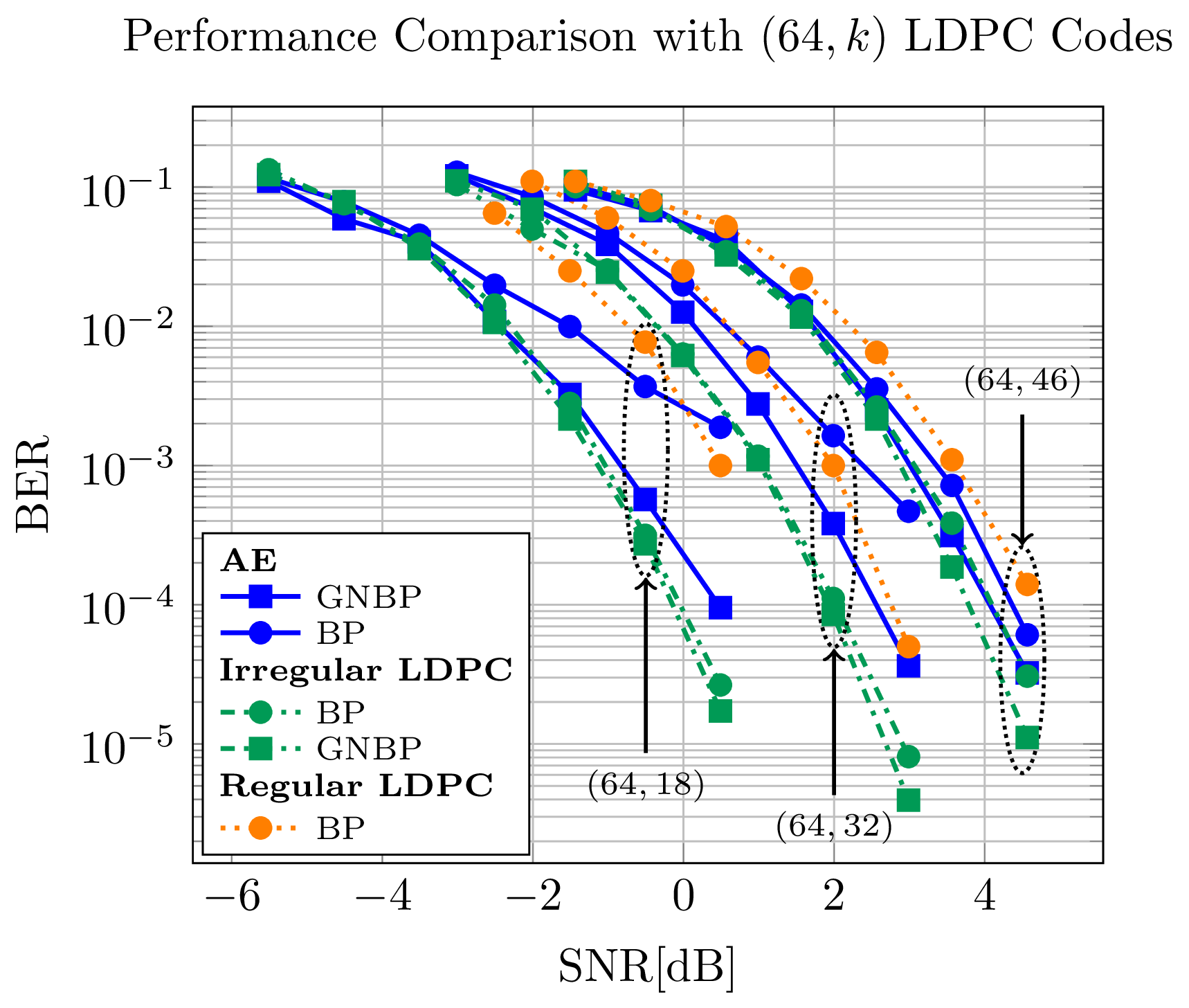
To ensure a fairer study of the proposed system, and since BP decoders were originally engineered to decode such codes, a comparison with LDPC codes of size 64 and with various rates is made (Fig. 15). The different regular and irregular LDPC codes are generated by the Progressive Edge Growth (PEG) algorithm [37] and decoded using BP ([plot:6418LDPCBP] / [plot:6418RegLDPCBP]) and GNBP ([plot:6418LDPCGNBP]) decoders. Said codes are compared with the proposed AE model trained with a GNBP decoder and evaluated with both BP ([plot:6418AEGNBPBP]) and GNBP ([plot:6418AEGNBP]) decoders. When considering a GNBP decoder, and despite the standard form constraint, the AE shows decent performances compared to the LDPC codes. AE performs significantly better than regular LDPC codes and is not far from the irregular codes (half a dB difference in the worst case). For the \(\frac{46}{64}\) code rate, the GNBP AE even reaches the performance of the irregular LDPC code under BP decoding and is close to the performance of the same code under GNBP decoding. Under BP decoding, the AE code is not as good as before, especially for the lower code-rates, where the systematic part of the PC matrix becomes prominent.
Comparison with State-of-the-Art (128,64) Codes - Impact of the Number of Iterations
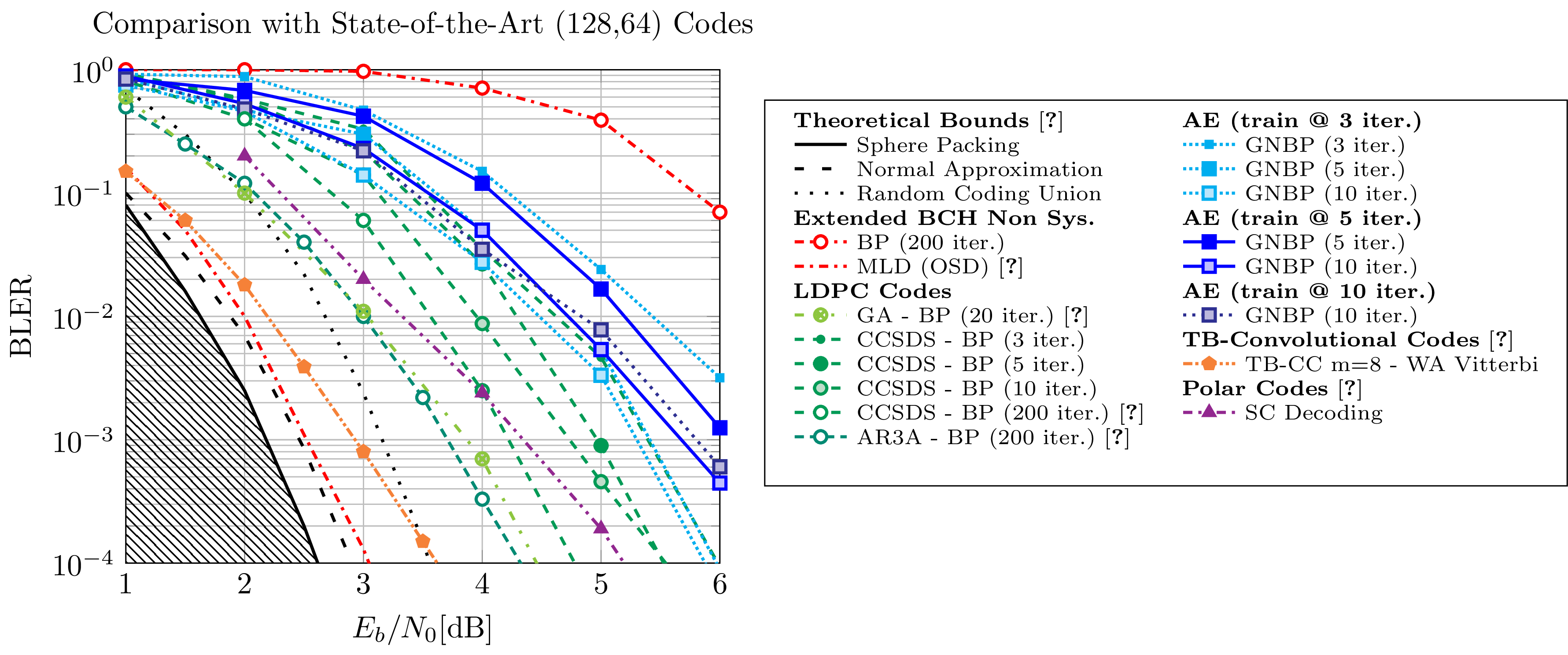
Finally, the AE is compared at the challenging (128,64) size to binary codes and theoretical bounds from [38] (Fig. 16). The model is trained and evaluated with a number of decoding iterations ranging from 3 to 10 to study the impact of the latter on the performance. When the number of iterations at evaluation is different from the one used during training, the GNBP decoder is re-trained while keeping the previously learned code fixed. AR3A ([plot:12864AR3ALDPC]) and CCSDS ([plot:12864CCSDLDPC]) LDPC codes [38] display better performance than the best AE GNBP ([plot:12864AEGNBP3iter10iter]) but their decoding complexity is also higher with up to 200 decoding iterations. For a fairer comparison the CCSDS code [35] is decoded with 3 ([plot:12864CCSDSLDPCNSYSBP3iter]), 5 ([plot:12864CCSDSLDPCNSYSBP5iter]) and 10 ([plot:12864CCSDSLDPCNSYSBP10iter]) BP iterations, thus reducing the performance gap to half a dB, similar to the one observed between the AE and the LDPC codes of Section 5.5.1. As expected the performance of the standard and the AE codes improves with the number of iterations. The number of training iterations of the AE also seems to have an impact on the final performance. Fig. 16 shows that it seems better to train the AE with 3 iterations and subsequently evaluate it with 10 ([plot:12864AEGNBP3iter10iter]) instead of training it with 10 iterations from the start ([plot:12864AEGNBP10iter]). Another ML-based approach relying on a GA is proposed as an additional comparison, although it uses 20 iterations ([plot:12864GA]) [21]. The latter performs well both against standard LDPC and the AE. However, the GA approach is fundamentally different from the one adopted in this paper because it attempts to optimize LDPC codes based on existing distributions while the AE learns ex nihilo. Although their decoding complexity is not easily comparable to that of the AE, the performance of a Polar code ([plot:12864PolarSC]) and a TB-CC ([plot:12864TBCCm8]) with their respective decoders are also provided [38]. Finally, the performance of an extended BCH is provided, showing poor BP performance ([plot:12864ExtBCHNSYSBP200iter]) even though its MLD performance ([plot:12864ExtBCHNSYSMLDOSD]) is close to the optimum. As before, the AE outperforms the BCH with a significantly reduced complexity. These results demonstrate that a systematic LBC of significant size can be learned by a ML procedure, with performance relatively close to that of LDPC codes and a controlled complexity.
Discussion, Conclusion & Perspectives
The AE architecture proposed in this paper is a performing, low complexity, AI-based approach for the joint design of small-to-medium size LBC and associated weighted decoders. Instead of improving the decoding procedure of codes that otherwise suffers from defects w.r.t. the targeted decoder, the proposed model supports the joint design of a LBC tailored to a BP-like decoding allowing significant performance gain. The main advantages of the approach are:
Code agnostic: The proposed approach does not require the knowledge of any LBC scheme from the literature, which allows to build codes of arbitrary size and rate.
Repeatable: The proposed architecture offers a repeatable training procedure. The study showed results within a 0.5 dB margin over 50 runs for a (31,16) code in Section 5.2.
Adaptable: The AE model can be trained with various decoders, e.g BP or GNBP. While GNBP has been shown to improve decoding performance on some codes, this study pointed out in Section 5.3 that the AE trained with a BP decoder can have performance close to that of the AE trained with the GNBP. Although it has not been confirmed in Section 5.4, a well designed code might thus not necessarily need a weighted decoding procedure.
Interpretable & Low complexity: The tightly structured architecture ensures a controlled number of parameters, tractable training procedure and high interpretability compared to black-box ML-based approaches. After training, the code’s matrices can be extracted and eventually used within a standard LBC decoder ensuring retro-compatibility with legacy, non AI-based, communication systems, with satisfying level of performance.
Scalable & Differentiable: As explained in Section 5.4, the structured design of both encoder and decoder is a key enabler for the scalability of the approach. The model is able to jointly learn a code and associated decoder only using the \(k\) basis vectors of the information space, while generalizing well to the many other unseen words even on relativity important code size. Moreover, the different structures presented throughout the paper ensure the differentiability of the complete architecture.
Efficient: The study of Section 5.4 showed improvement in terms of performance to complexity ratios when compared to other approaches, e.g. NBP or high performance but high complexity parallel decoders applied to (63,45) and (63,36) BCH codes. As shown in Section 5.5, the performance of the learned codes with size up to \((128,64)\) are close to those of LDPC codes, which are reference codes for BP decoding procedure. This emphasizes the ability of an AI-based system to design competitive LBC.
Still, several perspectives of future works can be outlined from the current proposition:
The current architecture does not exploit the blind property of the decoder as described in [11]. Instead, a bridge model is used to keep the encoder and decoder matched during training, which makes distributed online learning procedures complex in addition to limiting the codes to standard forms only. The latter usually leads to denser PC matrices which can be a limitation in terms of performance and decoding complexity when considering BP decoders. As such, it would be interesting to further study a non systematic AE architecture.
The GNBP RNN cell uses a low complexity static decoding strategy which repeat a certain number of time the BP operations under the same set of shared parameters. The decoding performance could be improved by dynamically computing the decoding graph at each decoding iterations of the RNN, based on the inputs and states of the decoder as it is often the case in standard RNN-based approaches. One could learn codes permutations to be applied during the decoding procedure, or inhibit certain parts of the graph, which has been shown to improve significantly decoding performance in parallel decoders [26], [27],[39].
A (GN)BP decoder was considered in this paper but lower complexity decoders from the literature e.g. MS, OMS or NOMS, could probably be used within the proposed system to further reduce the complexity of the system while maintaining competitive performance.
As shown in Section 5.2.4, the learned codes have unexpected degree distributions with high degrees. Further studies are needed to understand the performance of these distributions.
Acknowledgments
Thanks to E. Nachmani for the additional details on their results awsell as for providing us with the the codes matrices from their experimentations, used in Section 5.4. Thanks also to V. Savin for providing us with the reference short LDPC codes used in Sections 5.5.
This sub-section adopts with minor changes the same explanations as in a previous publication [11].↩︎
In this publication, results are presented, unless otherwise specified, in BER versus \(E_b/N_0\) [dB] where \(N_0/2\) is the variance of the (real) AWGN noise. When the proposed model is compared with other algorithms such as standard BP or NBP algorithms, 5 decoding iterations are considered, unless expressly stated otherwise.↩︎
Unless otherwise specified, the MLD decoders considered in this paper are based on an exhaustive minimal distance algorithm.↩︎
More precisely, the coding gain is normalized based on the number of multiplications. Such operations are usually considered to be more costly than additions. Moreover, the number of additions is unchanged between BP, GNBP and NBP decoders.↩︎