Blind Neural Belief Propagation Decoder for Linear Block Codes
Orange Institut Polytechnique de Paris
June 11, 2021
2021 Joint European Conference on Networks and Communications & 6G Summit (EuCNC/6G Summit) - 10.1109/EuCNC/6GSummit51104.2021.9482479
Copyright Notice: 2021 IEEE. Personal use of this material is permitted. Permission from IEEE must be obtained for all other uses, in any current or future media, including reprinting/republishing this material for advertising or promotional purposes, creating new collective works, for resale or redistribution to servers or lists, or reuse of any copyrighted component of this work in other works.
This work has been partly funded by the European Commission through the H2020 project Hexa-X (Grant Agreement no. 101015956).
Abstract
Neural belief propagation decoders were recently introduced by Nachmani et al. as a way to improve the decoding performance of belief propagation iterative algorithm for short to medium length linear block codes. The main idea behind these decoders is to represent belief propagation as a neural network, enabling adaptive weighting of the decoding process. In the present paper an efficient recurrent neural network architecture, based on gating and weights sharing mechanisms, is proposed to perform blind neural belief propagation decoding without prior knowledge of the coding scheme used by the encoder. The proposed architecture is able to learn to decode BCH (15,11) and BCH (15,7) codes and significantly improves the decoding performance over a standard belief propagation algorithm. A particular emphasis is given to the interpretability and complexity of the proposed model to ensure scalability to larger codes.
Introduction
Low-Density Parity Check (LDPC) codes were chosen in 5G-NR standard along with polar codes. For high code length, LDPC are a class of linear block codes associated with efficient and performing iterative decoding algorithms. Nonetheless, several use-cases, such as low power IoT, cannot use large codes because of the complexity of their decoding and their inadequacy with the relatively small payloads encountered. For shorter code length, the parity check (PC) matrix of LDPC codes is, unfortunately, no more sparse; "Low Density" property is lost and it becomes unavoidable to have short cycles in the PC matrix. As a consequence, performance of decoding algorithm based on Belief Propagation (BP), also known as Sum-Product (SP), becomes degraded. In such context, Nachmani et al. proposed to represent the BP algorithm as a Neural Network (NN), therefore enabling adaptative weighting of the messages exchanged during the decoding process [1]. The authors showed in simulations that this so called Neural Belief Propagation (NBP) approach improves the decoding performance for short to medium block-length codes. Yet, NBP algorithm assume a perfect knowledge of the code by the receiver to define the NN architecture. In the present paper, a novel NN architecture is proposed to perform blind NBP decoding of linear block codes without prior knowledge of the coding scheme used. Several publications discussed improvements of NBP using pruning [2], [3], weights sharing [4] or active sampling [5] but, to the best of our knowledge, this paper is the first to propose learning of NBP for linear block codes without knowledge of the code. Proposed structured architecture relies on gating and weights sharing mechanisms, ensuring reduced complexity, improved explainability, scalability and possibly better generalization capabilities for larger codes [6], [7].
The paper is structured as follows: Section 2 provides the theoretical background that will be used throughout the rest of the paper. Section 3 thoroughly describes the main contribution of this paper: an efficient gated Recurrent Neural Network (RNN) architecture for blind NBP decoding. Section 4 describes an implementation example of the proposed architecture for BCH (15,7) and BCH (15,11) codes as well as simulated Frame Error Rate (FER) demonstrating that the NN model learns to decode, performing at least at the level of a standard BP algorithm and eventually outperforming it thanks to NBP approach. Finally, Section 5 gives the conclusions of the study and perspectives for future works.
Notations: Matrix are denoted as \(\mathbf{M}\), vector as \(\mathbf{v}\) and scalar as \(s\). Hadamard product is denoted as \(\odot\). \(\mathrm{diag}(\mathbf{v})\) denotes a diagonal matrix with vector \(\mathbf{v}\) as main diagonal.
Theoretical Background
A linear block code \(\mathcal{C}\) of length \(n\) and rank \(k\) is considered. The associated generator matrix of size \(k \times n\) and corresponding PC matrix of size \((n-k) \times n\) are denoted as \(\mathbf{G}\) and \(\mathbf{H}\) respectively. The PC matrix can be represented as a bipartite graph model called a Tanner Graph [8], a certain type of Factor Graph (FG). Such representation enables efficient iterative decoding based on classic message passing algorithms such as the BP. This algorithm aims to converge to the transmitted code-word by iteratively exchanging "beliefs" between the nodes of the graph on the probable values of received code-word bits. Usually, exchanged messages are related to the Log-Likelihood Ratios (LLR) of the received bits and the sum-product update rule can be applied to the different nodes using the following equations (see [9] for more details):
SP update rule applied at variable node \(i\) to compute message toward the check node \(j\): \[\mu_{v_i c_j} = \lambda_i + \sum_{k \neq j}{\mu_{c_k v_i}} \label{eq:sum}\] Where \(\lambda_i\) is the a priori LLR received by variable node \(i\) and \(\mu_{c_k v_i}\) are the messages received by variable node \(i\) from neighboring check nodes \(k\).
SP update rule applied at check node \(j\) to compute message toward the variable node \(i\): \[\mu_{c_j v_i} = 2 \times \mathrm{arctanh} \left[ \prod_{k \neq i} \mathrm{tanh}\left(\frac{\mu_{v_k c_j}}{2}\right)\right] \label{eq:product}\] Where \(\mu_{v_k c_j}\) are the messages received by check node \(j\) from neighboring variable nodes \(k\).
SP update rule applied at variable node \(i\) to compute the bit \(i\) a posteriori LLR: \[\widetilde{\lambda_i} = \lambda_i + \sum_{k}{\mu_{c_k v_i}} \label{eq:out}\]
The FG not being cycle-free, it is necessary to apply iterative decoding by passing messages back and forth between variable and check nodes, using equations [eq:sum] and [eq:product], before hopefully converging to a satisfying solution. NBP algorithm [1] proposes to learn how to weight messages and input LLR of equations [eq:sum], [eq:product] and [eq:out], to reduce the negative influence of the short cycles on the final decoding performance.
Blind NBP as an efficient gated RNN
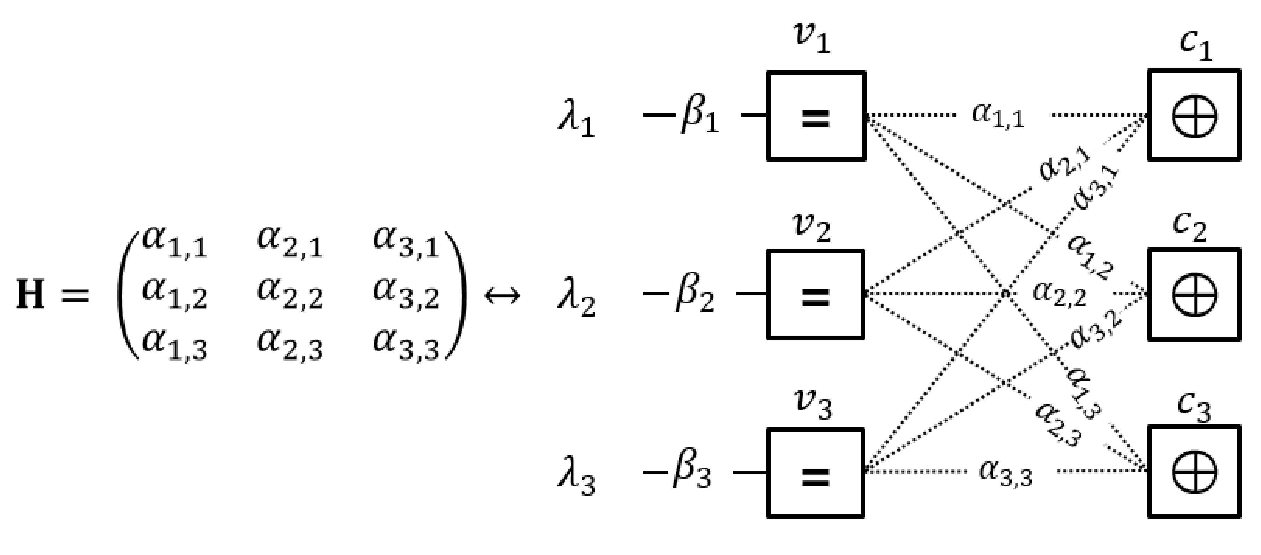
In this paper, a NN architecture is proposed to perform blind NBP algorithm applied to the decoding of linear block codes. In the proposed method, receiver no longer requires prior knowledge of the used coding scheme. As a consequence, it needs to learn both the factor graph topology and the weights of the NBP. The proposed decoder is based on a custom Recurrent Neural Network (RNN) cell architecture that leverages weight sharing and gating mechanisms. At first, SP rules will be described as efficient matrix operations for generic linear block codes. Then the proposed operations will be embedded in a RNN cell architecture. Mechanisms enabling an efficient decoding scheme to be learned will be described. A generic factor graph associated with an hypothetical \(3\times3\) PC matrix as described in Fig. 1 will be used throughout this paper to illustrate the proposed architecture.
Variable to check nodes
At each NBP iteration the decoder starts by updating messages from variable to check nodes \(\mu_{v_i c_j}\) following a weighted version of Eq. [eq:sum] (The input messages received from check nodes \(\mu_{c_j v_i}\) are initialized to 0 at the first iteration). This computation can be implemented using a dense NN layer as shown in Fig. 2. \(\omega(\alpha_{i,j})\) is a non-linear function applied to the parameters of the FG to represent both gating (i.e. binary selection) and weighting mechanisms. For example, if \(\omega(\alpha_{i,j})\) is defined as a step function, then the computational graph will reproduce a standard BP algorithm, with binary weights. The \(\beta_i\) coefficients, do not need to go through \(\omega\) function because there is no interest in pruning any of the inputs.
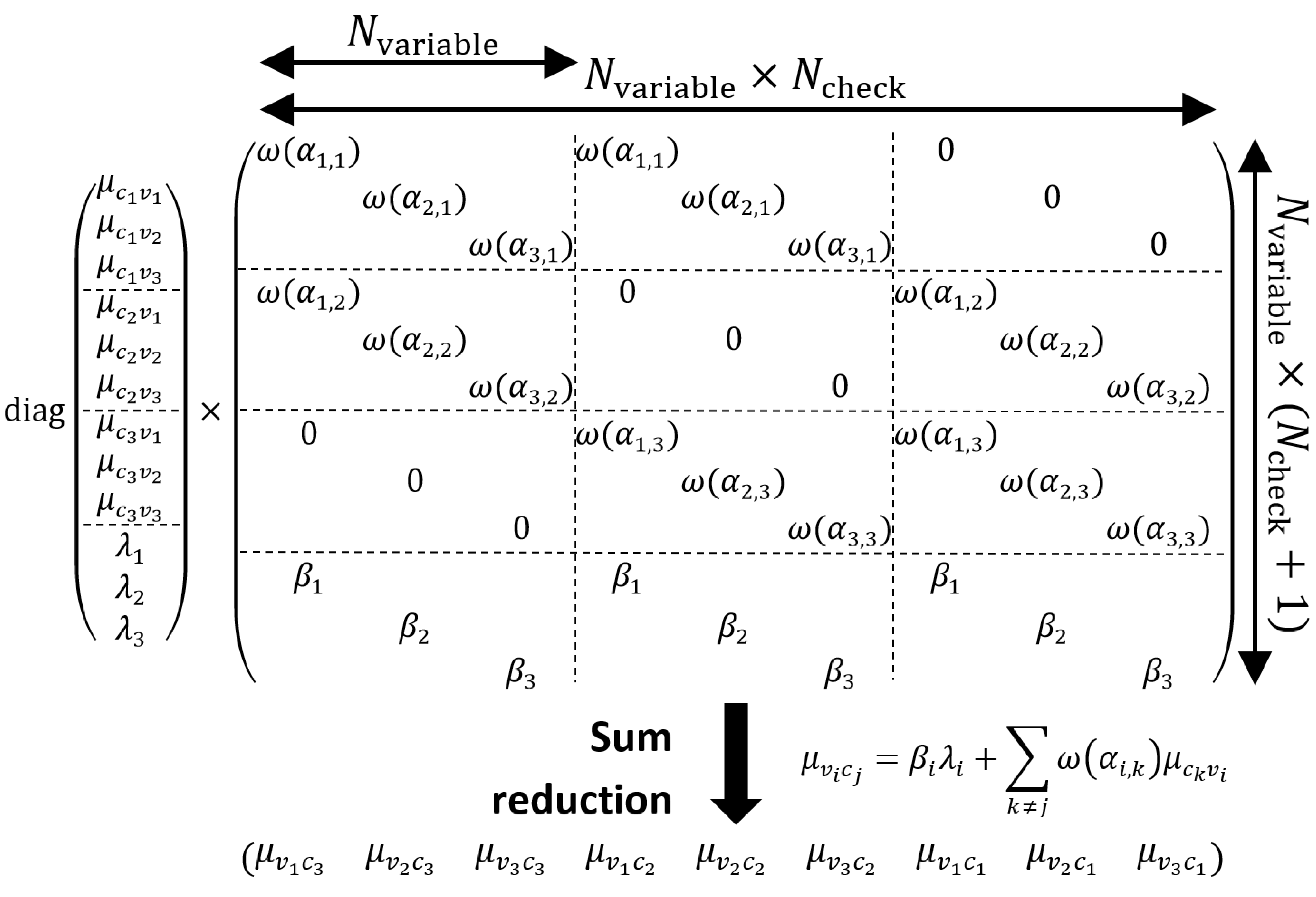
With a good initialization of the parameters, this layer can rigorously perform the update rule for messages from variable to check nodes, but it has several drawbacks:
High complexity in terms of number of parameters and computations.
Need of a sparse weights matrix to actually perform BP algorithm.
Loss of explanability after a training. There are no guarantees that the performed algorithm is still a BP or NBP (without further refinements, all parameters, even zeros, being trainable).
Low generalization capabilities due to loosely structured architecture [6], [7] leading to probable unscalability to bigger codes.
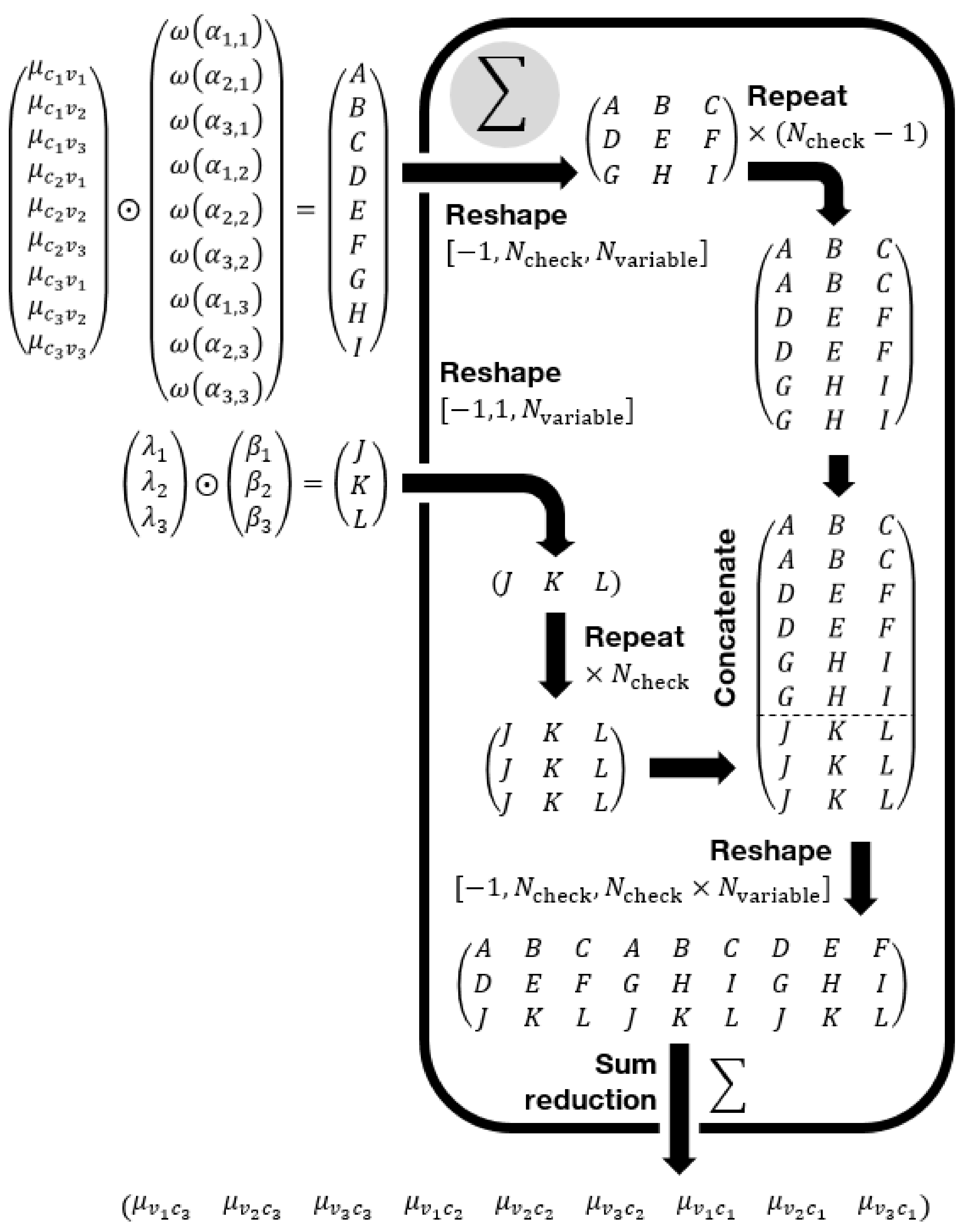
An efficient, scalable and fully differentiable computational graph for the variable to check nodes update rule is proposed in this work as shown in Fig. 3. This graph drastically reduces the number of parameters and operations as shown in Table 1 and ensures that a NBP is executed1.
| DENSE (Fig 2) | IMPROVED (Fig 3) | |
|---|---|---|
| # multiplications | \(\mathcal{O}(N_{\mathrm{var}}^2 \times N_{\mathrm{check}}^2)\) | \(\mathcal{O}(N_{\mathrm{var}} \times N_{\mathrm{check}})\) |
| # additions | \(\mathcal{O}(N_{\mathrm{var}}^2 \times N_{\mathrm{check}}^2)\) | \(\mathcal{O}(N_{\mathrm{var}} \times N_{\mathrm{check}}^2)\) |
| Biggest tensor allocation | \(\mathcal{O}(N_{\mathrm{var}}^2\times N_{\mathrm{check}}^2)\) | \(\mathcal{O}(N_{\mathrm{var}} \times N_{\mathrm{check}}^2)\) |
Check to variable nodes
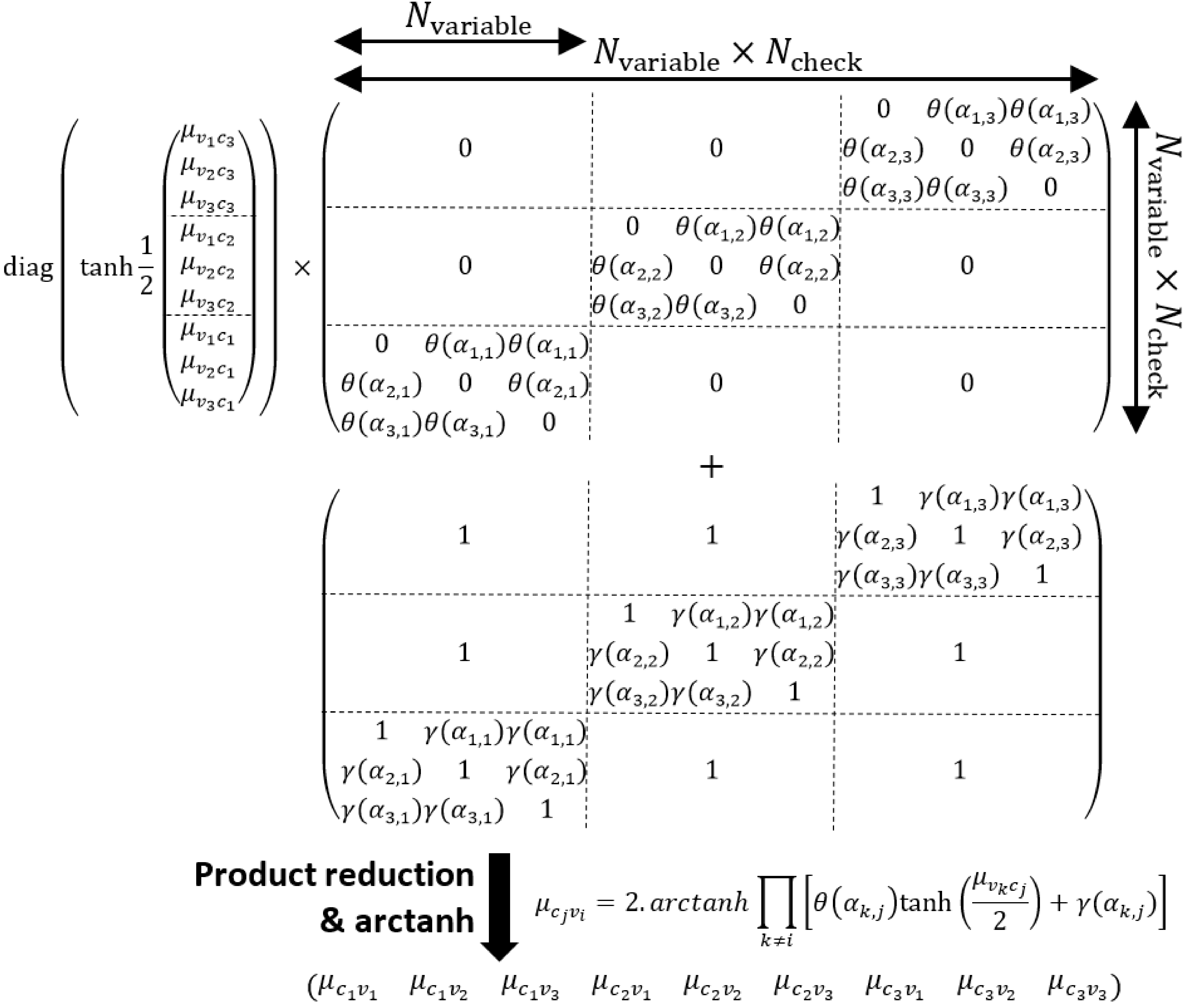
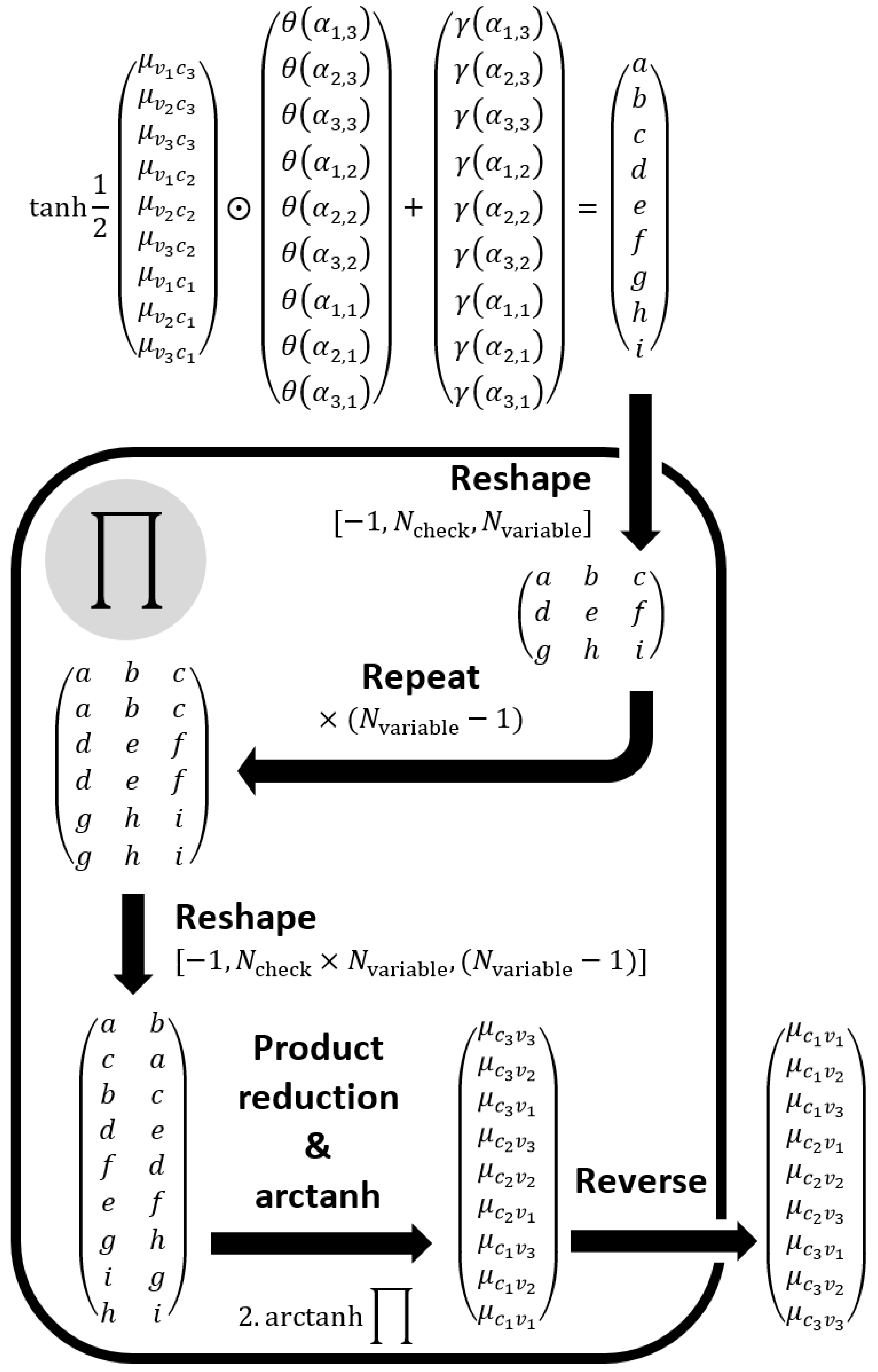
The second step of the NBP decoding process consists in updating messages from check to variable nodes \(\mu_{c_j v_i}\) using a weighted version of Eq. [eq:product]. It can be implemented by using a naive architecture based on a few differentiable operations as described in Fig. 4. The multiplicative step selects and weights the inputs. The additive step ensures the neutral element of the product is added to non-selected inputs, before the upcoming product reduction. The following \(\mathrm{arctanh}\) activation function having exploding gradient when approaching -1 or +1 makes gradient based training difficult. To overcome this issue one can use a Taylor expansion of the function as proposed in [10]. \(\theta(\alpha_{i,j})\) and \(\gamma(\alpha_{i,j})\) are non-linear functions applied to the parameters of the FG. For example, to apply a standard BP algorithm, one can choose: \[\begin{aligned} &\theta(\alpha_{i,j})=\rm{step}(\alpha_{i,j})&\mathrm{ and }&&\gamma(\alpha_{i,j})=1-\rm{step}(\alpha_{i,j})\\ \end{aligned}\]
A judicious parameterization of this architecture implements the update rule for messages from check to variable nodes. But, once again, it is inefficient and can lose explainability after a training phase. An efficient computational graph for this update rule is proposed in Fig. 5. Based on standard matrix operations, it reduces the complexity as shown in Table 22.
| DENSE (Fig 4) | IMPROVED (Fig 5) | |
|---|---|---|
| # multiplications | \(\mathcal{O}(N_{\mathrm{var}}^2 \times N_{\mathrm{check}}^2)\) | \(\mathcal{O}(N_{\mathrm{var}}^2 \times N_{\mathrm{check}})\) |
| # additions | \(\mathcal{O}(N_{\mathrm{var}}^2 \times N_{\mathrm{check}}^2)\) | \(\mathcal{O}(N_{\mathrm{var}} \times N_{\mathrm{check}})\) |
| Biggest tensor allocation | \(\mathcal{O}(N_{\mathrm{var}}^2\times N_{\mathrm{check}}^2)\) | \(\mathcal{O}(N_{\mathrm{var}}^2 \times N_{\mathrm{check}})\) |
Output
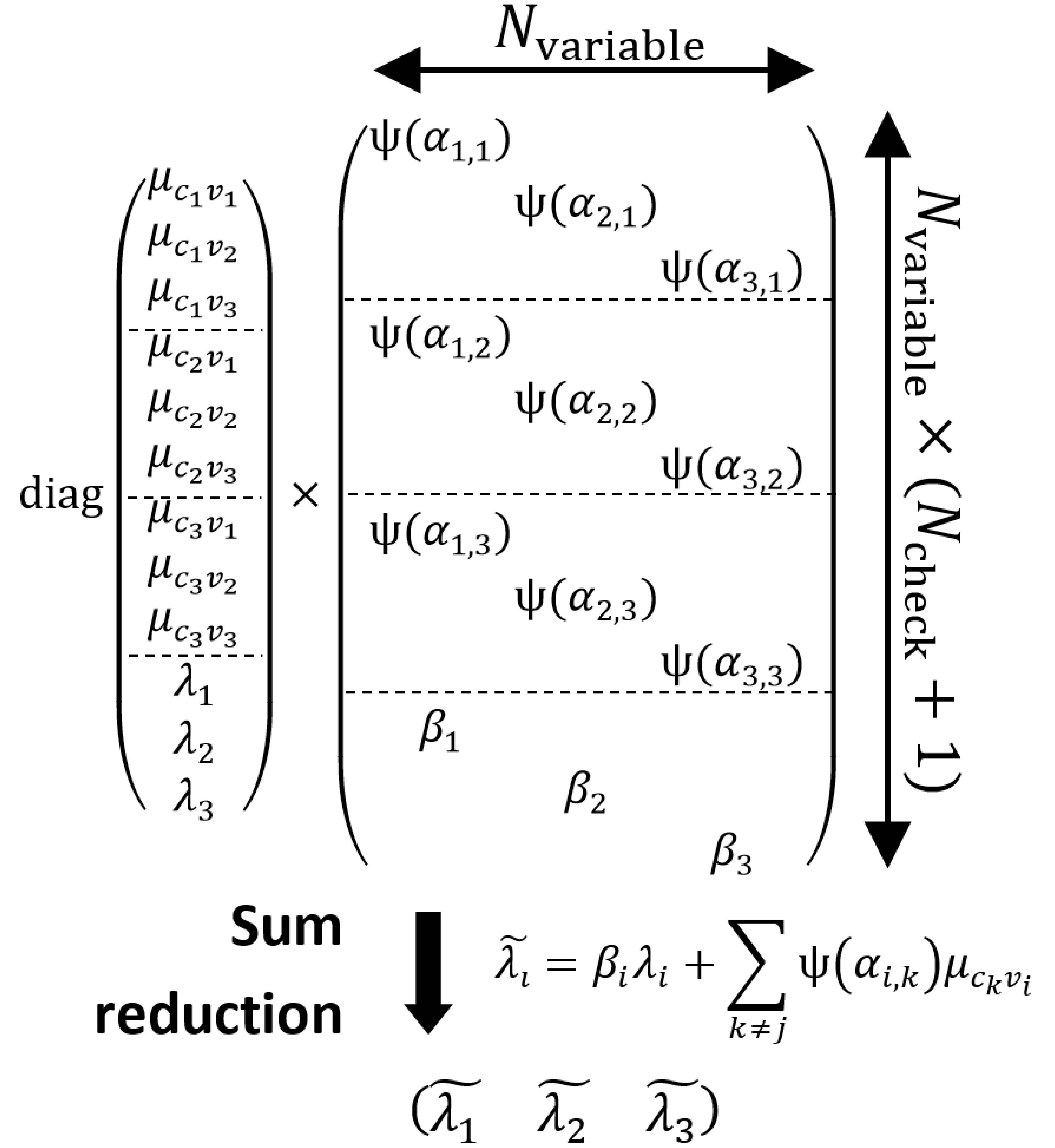
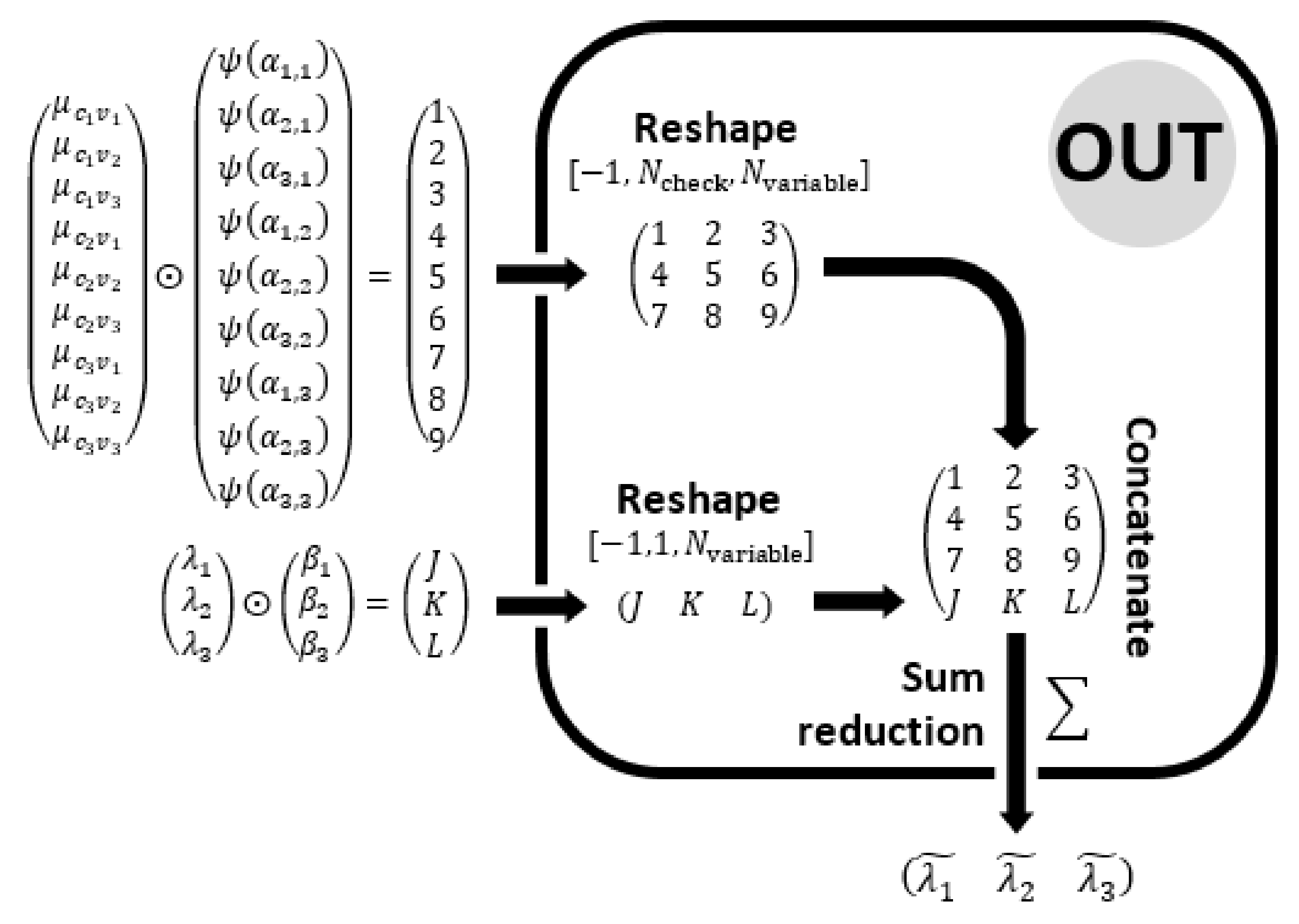
The final step of the NBP decoding consists in computing the a posteriori LLR \(\widetilde{\lambda_i}\) using a weighted version of Eq. [eq:out]. Similarly to Section 3.1, one can express this computation as a simple dense layer as shown in Fig. 6. A more efficient computational graph is proposed on Fig. 7. The complexity of the proposed model is reduced compared to the dense architecture as described in Table 3.
| DENSE (Fig 6) | IMPROVED (Fig 7) | |
|---|---|---|
| # multiplications | \(\mathcal{O}(N_{\mathrm{var}}^2 \times N_{\mathrm{check}})\) | \(\mathcal{O}(N_{\mathrm{var}} \times N_{\mathrm{check}})\) |
| # additions | \(\mathcal{O}(N_{\mathrm{var}}^2 \times N_{\mathrm{check}})\) | \(\mathcal{O}(N_{\mathrm{var}} \times N_{\mathrm{check}})\) |
| Biggest tensor allocation | \(\mathcal{O}(N_{\mathrm{var}}^2\times N_{\mathrm{check}})\) | \(\mathcal{O}(N_{\mathrm{var}} \times N_{\mathrm{check}})\) |
RNN cell
BP decoding being an iterative algorithm, the aforementioned operations must be repeated several times to reach good performance. RNN can be used to execute such iterative decoding in a NN framework [1]. Using the previously described operations, a structured RNN cell tailored to perform blind NBP decoding of linear block codes is proposed in Fig. 8. The RNN cell, inspired by gated cells such as LSTM [11] or GRU [12], is built around two types of trainable weights:
Gating weights: \(\mathbf{w_G}\) represent the topology of the FG and are used to select messages accordingly during the different steps of the decoding process. To represent such binary selection behavior a sigmoidal activation function \(\sigma\) is applied to these weights.
NBP weights: The \(\mathbf{w_\Sigma}\) and \(\mathbf{w_{OUT}}\) weights are used to improve the performance of the decoding scheme similarly to the NBP mechanism described in [1]. They should be real valued and centered around 1 to ensure weighting of the messages and not selection.
All the weights are shared between different RNN iterations (following known properties of RNN). Gating weights are also distributed inside any given iteration between the different operations of the BP algorithm; see Fig. 8. The structured NN architecture ensures the learned decoding algorithm is similar to a NBP but allows the learning of the code’s factor graph’s topology. In the proposed architecture, the aforementioned functions \(\omega\), \(\theta\), \(\gamma\) and \(\psi\) can be defined as follows:
\[\begin{aligned} \omega(\boldsymbol{\alpha})&=\mathbf{w_\Sigma}\odot\sigma\left(\mathbf{w_G}\right)&\psi(\boldsymbol{\alpha})&=\mathbf{w_{OUT}}\odot\sigma\left(\mathbf{w_G}\right)\\ \theta(\boldsymbol{\alpha})&=\sigma\left(\mathbf{w_G}\right)&\gamma(\boldsymbol{\alpha})&=1-\sigma\left(\mathbf{w_G}\right)\\ \end{aligned}\]
The gate mechanism selects messages using a "refined gate function" \(\sigma\left(\mathbf{w_G}\right)\) [13]. This function closely acts as a sigmoid function but allows better gradient back-propagation in the saturation regime of the sigmoid thus improving the learn-ability of the gates (at the cost of additional trainable parameters). It can be noted that the chosen architecture only weights the messages at certain steps. From conducted experiments, using different weights before \(\mathbf{\Sigma}\) and OUT operations seems performing. In most of the trials, using weights before the \(\mathbf{\Pi}\) operation was detrimental to the performance of the model. This might partially be explained by the numerical sensitivity of the product reduction and \(\mathrm{arctanh}\) function used in \(\mathbf{\Pi}\) block. The weighting of the input LLR (using \(\boldsymbol{\beta}\) weights) did not prove efficient either.
Experimental setup and results
System model
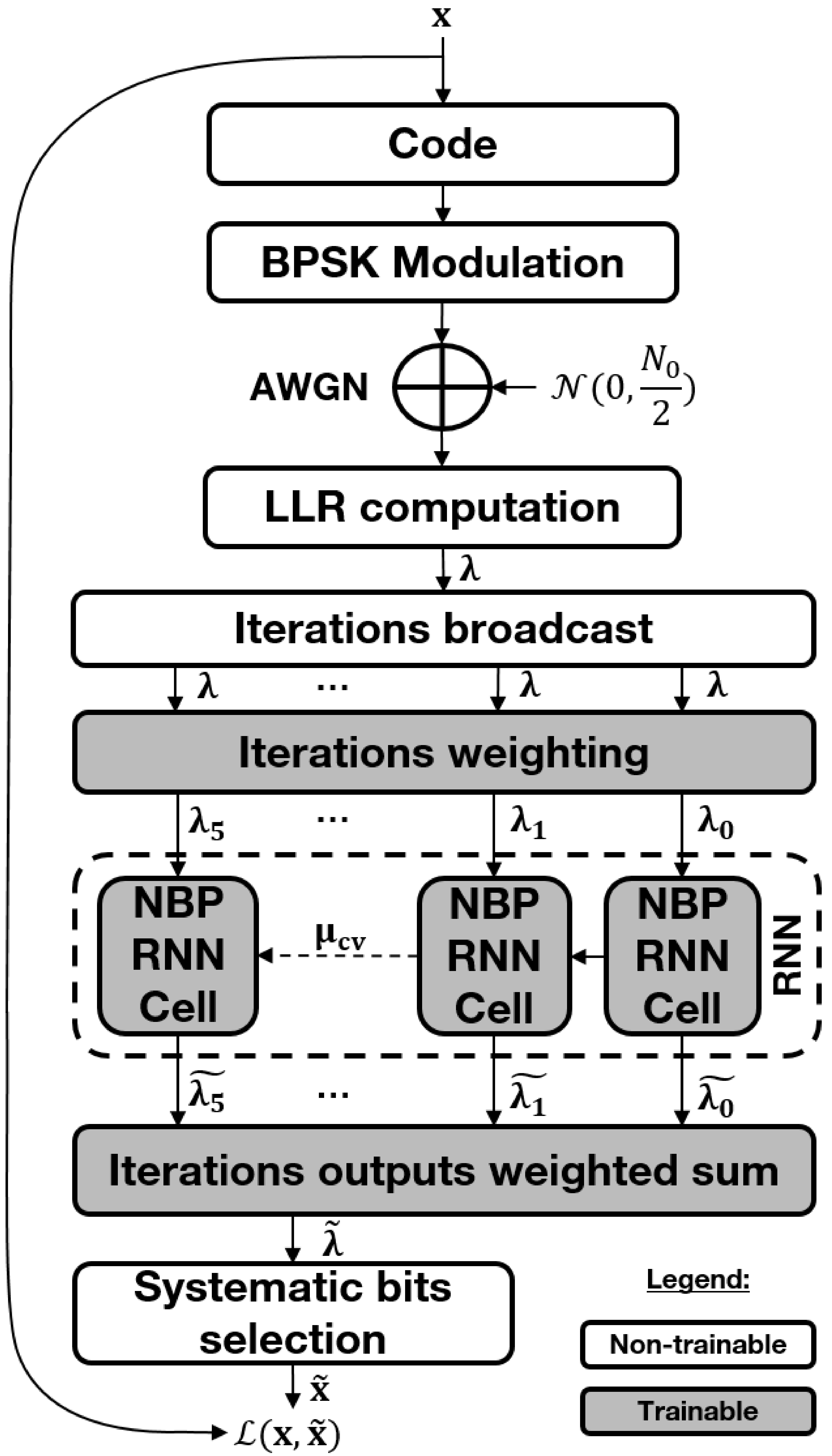
To evaluate the performance of the proposed RNN cell, an end-to-end NN model is defined in TensorFlow with the following custom layers (see Fig. 9):
Code: Information words \(\mathbf{x}\) are encoded using systematic versions of either BCH (15,11) or BCH (15,7) codes described in [14].
Modulation: A BPSK modulation is applied.
Channel: Symbols go through an AWGN channel.
Soft demodulation: Given the modulation and channel used, LLR of the received samples are computed.
LLR pre-processing: To facilitate the training of the RNN, the LLR are normalized to \(\left[-1,+1\right]\) range according to the maximum absolute LLR in each code-word. The LLR are then broadcasted as many times as BP iterations needed (in this study, this number is fixed to 5). An iteration-wise weighting mechanism is applied to the normalized code-words. This might allow the NN to compensate for inadequate normalization range of the code-words on one hand, and also introduce variability in the RNN iterations by changing the balance between inputs LLR and messages from previous iteration, on the other hand.
Decoding: The proposed Gated NBP RNN Cell is used to decode the received code-words. As emphasized previously, the blind NBP has to learn the coding scheme used at the emitter.
Outputs processing: Instead of extracting only the result of the last BP iteration, the outputs of all iterations are re-combined using a weighted sum. Thus, the RNN layer is used in a "many-to-many" configuration. This approach is inspired by [4], [15] and might allow an easier back-propagation of the gradient by injecting it back at each BP iterations. This also allows the system to give more importance to the iteration outputs that are most reliable from training experience. Knowing the position of the systematic bits of the code, a deterministic selection layer is then applied to select these bits and a sigmoid function is applied to squeeze decoded LLR to either 0 or 1.
For both codes, the overall complexity of the model is described in Table 4.
| Weights | # Trainable Parameters | BCH(15,7) decoder | BCH(15,11) decoder |
|---|---|---|---|
| PRE-PROCESSING STAGE | |||
| Iteration weights | \(N_{\mathrm{Iter}}\) | 5 | 5 |
| NBP RNN | |||
| \(\mathbf{w_G}\) | \(N_{\mathrm{Var}} \times N_{\mathrm{Check}}\) | 120 | 60 |
| Refine Gate \(\sigma\) | \(2 \times N_{\mathrm{Var}} \times N_{\mathrm{Check}}\) | 240 | 120 |
| \(\mathbf{w_\Sigma}\) | \(N_{\mathrm{Var}} \times N_{\mathrm{Check}}\) | 120 | 60 |
| \(\mathbf{w_{OUT}}\) | \(N_{\mathrm{Var}} \times N_{\mathrm{Check}}\) | 120 | 60 |
| POST-PROCESSING STAGE | |||
| Iteration Out Weights | \(N_{\mathrm{Iter}}\) | 5 | 5 |
| TOTAL | \(2 \times N_{\mathrm{Iter}} + 5 \times N_{\mathrm{Var}} \times N_{\mathrm{Check}}\) | 610 | 310 |
Training
The auto-encoder framework enables a simple training process as the loss function can be computed as the binary cross-entropy between initial information words \(\mathbf{x}\) and decoded words \(\mathbf{\widetilde{x}}\). For both codes, training is performed using randomly chosen information bits, divided in words of size \(k\). The number of words used for training corresponds to 10 times the total number of possible words, \(2^k\). The SNR used during training phase is fixed at 4 dB. RMSProp optimizer is used with a triangular cyclic learning rate scheduler [16] oscillating between learning rates of \(10^{-2}\) and \(10^{-1}\). The model is trained during 250 Epochs. Except \(\mathbf{w_G}\) weights that are initialized using Glorot uniform initializer, all the other weights are initialized to 1. A shifted \(\ell_2\) regularization mechanism is applied to penalize learned NBP weights that lie too far from 1. The main focus of the paper being to provide a working architecture for blind NBP decoding, several improvements could be brought to the training process and hyper-parameters choices in future works.
Results
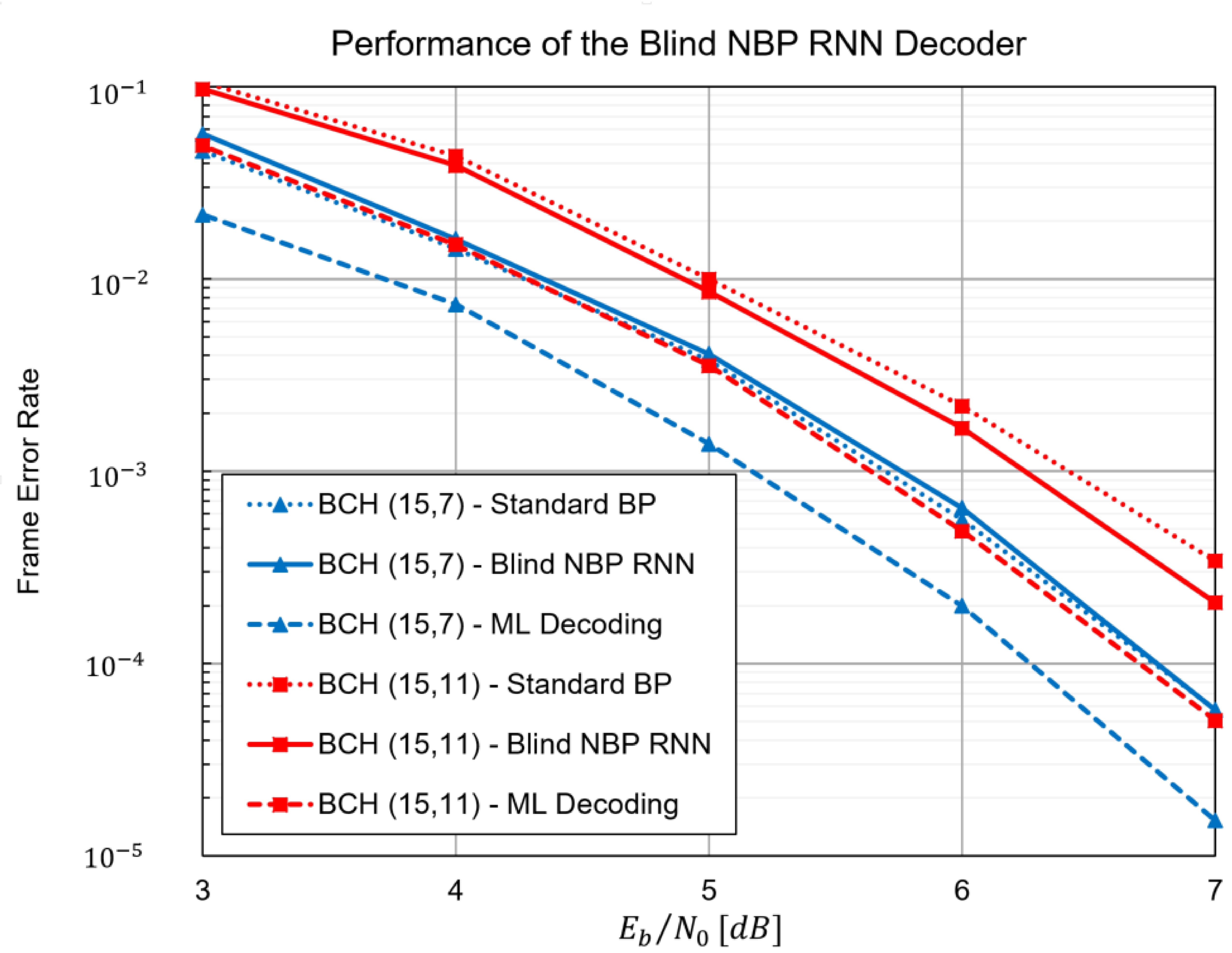
The model was evaluated on a dataset composed of randomly chosen words. To obtain reliable results, instead of fixing the number of testing words, the number of errors to reach has been fixed. The performance of the best model among 50 trainings, denoted as "Blind NBP RNN", is compared with Maximum Likelihood (ML) [14] and standard BP decoding baselines for both codes as depicted in Fig. 10. All the performance curves are displayed in frame error rate (number of code-words erroneously decoded among all the processed code-words). Proposed model is able to learn to decode both codes, without prior knowledge, at least at the level of performance of a standard BP decoder, and even outperforms it in the case of BCH (15,11) code thanks to NBP approach.
Conclusion and perspectives
In this paper an efficient gated RNN architecture has been introduced for the decoding of linear block codes. This architecture enables a blind approach where no prior knowledge of the used coding scheme is needed at the receiver side and leverages NBP technique to achieve potential performance gains over standard BP decoders.The computational graph has been designed to be low-complexity, generic and scalable to bigger codes. The main advantages of the proposition are:
Controlled number of trainable parameters and computations in the NN thanks to weights sharing and efficient computational graph.
Structured architecture ensuring the application of NBP algorithm for the decoding of linear block codes as well as improved explainability of the model.
Potential performance gains over standard BP decoders thanks to the application of a NBP like approach.
Improved decoder flexibility thanks to it’s training capabilities.
The proposed model was able to learn to decode BCH (15,11) and BCH (15,7) codes at least at the level of performance of a standard BP. Interesting leads for further works include the study of the generalization abilities of such structured architecture. This property is crucial to learn decoding scheme for bigger codes where it is not possible to provide all the code-words in the training dataset. This was in fact one of the insights behind the proposition of such architecture and the use of linear block codes. For online learning, the training repeatability of the model should also be improved as it sometimes, although rarely, fails to discover a competing decoding scheme compared to BP. Other initializers, pruning techniques, and different hyper-parameters could be envisioned to solve this problem. Finally, it would be of great interest to include this decoder in a fully trainable end-to-end architecture, to simultaneously discover efficient coding and decoding scheme. This last perspective, enabled by the proposed trainable blind NBP decoder, will be subject to further studies.
Function \(\omega\) is not included in the complexity table as it can be performed once for all the batch. If the reduction is performed in a continuous Multiply/Accumulate approach, the biggest tensor allocation can be reduced to \(\mathcal{O}(N_{\mathrm{var}}\times N_{\mathrm{check}})\) for the dense architecture↩︎
The algorithmic complexity of \(\mathrm{tanh}\) and \(\mathrm{arctanh}\) is not included in the table because of the presence of these operations in both architectures.↩︎