Low-Complexity Neural Networks for Baseband Signal Processing
Orange Institut Polytechnique de Paris Grenoble INP - Phelma
December 11, 2020
2020 IEEE Globecom Workshops, Taipei, Taiwan - 10.1109/GCWkshps50303.2020.9367521
Copyright Notice: 2020 IEEE. Personal use of this material is permitted. Permission from IEEE must be obtained for all other uses, in any current or future media, including reprinting/republishing this material for advertising or promotional purposes, creating new collective works, for resale or redistribution to servers or lists, or reuse of any copyrighted component of this work in other works.
Abstract
This study investigates the use of neural networks for the physical layer in the context of Internet of Things. In such systems, devices face challenging energy, computational and cost constraints that advocate for a low-complexity baseband signal processing. In this work, low-complexity neural networks are proposed as promising candidates. They present adaptability to operating conditions, high performance to complexity ratio and also offer a good explainability, crucial in most communications systems that cannot rely on "black-box" solutions. Moreover, recent advances in dedicated hardware for neural networks processing bring new perspectives in terms of efficiency and flexibility that motivate their use at the physical layer. To illustrate how classical baseband signal processing algorithms can be translated to minimal neural networks, two models are proposed in this paper to realize single-path equalization and demodulation of M-QAM signals. These models are assessed using both simulation and experimentation and achieve near optimal performances.
Introduction
In the context of 5G and beyond 5G communication systems, the use of Neural Networks (NN) at the physical (PHY) layer is of growing interest. Envisioned use cases are as varied as signal and modulation classification [1], coding and decoding [2], interference cancellation [3], joint channel estimation and symbol detection [4], and joint modulation and coding [5]. Two approaches are usually proposed in the literature. The first one, named functional approach, aims to replace existing processing blocks of a standard PHY layer by NN based algorithms [1], [6]. The second one, named End-to-End approach, addresses the question in a more ground-breaking way. The whole signal processing chain of both transmitter and receiver is redefined as one or more NN that learn a new communication scheme. This scheme is optimized with regard to a given channel and communication scenario [5]. This paper focus on the functional approach that is compatible with an implementation in current standards.
In both approaches, the design of NN architectures often follow empirical methods inherited from domains such as Computer Vision or Natural Language Processing, where NN showed impressive performance compared to handcrafted algorithms. Notable models, so called Deep Neural Networks (DNN), leverage several hidden layers to express sophisticated non-linear functions, solving complex problems which do not have any known analytical solution. A potential drawback of models with important number of parameters lies in the complex and time-consuming inference and learning processes. These limitations are usually incompatible with the energy, computational power and cost constraints of Internet of Things (IoT) and Green networks. Moreover, due to their inherent "black-box" design, DNN are often not explainable,
i.e.
they do not offer the analytical guarantees, and operational reliability, usually required in communication systems.
Therefore, this paper discusses the design of a NN based PHY layer with realistic implementation constraints, and advocates for the use of low-complexity NN, designed to have a minimal architecture regarding the problem to solve. Using such algorithms, particularly when supported by NN dedicated hardware, allow to leverage many advantages such as higher efficiency, lower energy consumption or better explainability. The aim of this study is to illustrate this approach with concrete examples.
This paper is structured as follows. Section 2 describes the system model used throughout the study. Section 3 exposes the main contributions of the paper and illustrates how the problems of single-path equalization and M-QAM demodulation can be expressed in terms of low-complexity and explainable NN architectures. Section 4 briefly addresses the question of the learning processes that may be involved in the configuration of such models. Section 5 presents an experimental evaluation of the aforementioned system using Software Defined Radio (SDR) and a channel emulator. The system achieves near-optimal Bit-Error Rate (BER) performance. Section 6 summarize the results of the study and explores some perspectives of using efficient NN for PHY layer, before concluding the paper.

System model
The communication system described in Figure 1 is considered. Random binary sequences are modulated using a Gray mapped M-QAM modulator. A single-path channel model is adopted and defined as its baseband equivalent. It is composed by the following combination of propagation effects and hardware impairments:
Additive White Gaussian Noise (AWGN): real and imaginary parts of the noise are sampled from a zero-mean Gaussian distribution1: \[\mathbf{n_k} = \begin{pmatrix} n_{i_k}&n_{q_k} \end{pmatrix}^{\rm{T}} \textrm{with } n_{i_k},n_{q_k} \overset{i.i.d}{\sim}\mathcal{N}\left(0,\,\sqrt{\rm{N_0}/2}\right)\]
Phase shift: symbols are rotated by an angle \(\phi\) with the following rotation matrix: \[\bf{R} = \begin{pmatrix} \phantom{-}\cos(\phi )& \sin(\phi )\\ -\sin(\phi )& \cos(\phi ) \end{pmatrix}\]
IQ amplitude imbalance: a different scaling factor is applied to I and Q channels as described in the following diagonal stretching matrix: \[\bf{A} = \textrm{diag} \begin{pmatrix} \alpha_i & \alpha_q \end{pmatrix}\]
IQ offset: a different offset is applied to I and Q channels: \[\mathbf{o} = \begin{pmatrix} \omega_i&\omega_q \end{pmatrix}^{\rm{T}}\]
Phase shift, IQ amplitude imbalance and IQ offset are considered constant under block-fading hypothesis2. The overall channel effect on a given sample is:
\[\mathbf{y_k}^{\rm{T}} = \mathbf{x_k}^{\rm{T}}\bf{RA} + (\mathbf{o} + \mathbf{n_k})^{\rm{T}} \label{channel_impairments}\] \[\begin{pmatrix} y_{i_k}\\ y_{q_k} \end{pmatrix}^{\rm{T}} = \begin{pmatrix} x_{i_k}\\ x_{q_k} \end{pmatrix}^{\rm{T}} \begin{pmatrix} \phantom{-}\alpha_i \cos(\phi )& \alpha_q \sin(\phi )\\ -\alpha_i \sin(\phi )& \alpha_q \cos(\phi ) \end{pmatrix} + \begin{pmatrix} \omega_i + n_{i_k}\\ \omega_q + n_{q_k} \end{pmatrix}^{\rm{T}} \nonumber \\ \]
where \(\mathbf{x_k}\) is the k-th input symbol and \(\mathbf{y_k}\) the corresponding sample, affected by the channel.
On the receiver side, the effect of the channel must be mitigated by a single-path equalizer. If perfect equalization is considered, one can obtain the equalized sample:
\[\mathbf{u_k} = \tilde{\mathbf{x_k}}+ \tilde{\mathbf{n_k}}\]
where \(\mathbf{u_k}\) is the equalized sample and \(\tilde{\mathbf{n_k}}\) is the noise sample after equalization that can be described, without loss of generality, as a bi-variate AWGN.
A decision process is finally applied to recover the transmitted binary code-words.
Low-complexity NN models for PHY layer
This section proposes two new low-complexity NN for baseband processing. They are described purely as deterministic mathematical models with an analytical derivation of their parameters. The question of Machine Learning (ML) and parameters optimization will be briefly addressed in section 4.
Designing a NN based single-path equalization system
This section illustrates how a simple NN can be used to perform a single-path equalization. The objective of the equalization block is to retrieve the original samples, before the channel impairments. The optimal solution given the channel impairments described in Equation [channel_impairments] is: \[\label{optimal_eq_scheme} \begin{aligned} \mathbf{u_k}^{\rm{T}} &= (\mathbf{y_k} - \mathbf{o})^{\rm{T}}(\bf{RA})^{-1} \\ &= \mathbf{y_k}^{\rm{T}}(\bf{RA})^{-1} - \mathbf{o}^{\rm{T}}(\bf{RA})^{-1}\\ &= \mathbf{x_k}^{\rm{T}} + \mathbf{n_k}^{\rm{T}}(\bf{RA})^{-1} \end{aligned}\]
where \[(\bf{RA})^{-1}= \frac{1}{\alpha_i\alpha_q} \begin{pmatrix} \alpha_q \cos(\phi )& -\alpha_q \sin(\phi )\\ \alpha_i \sin(\phi )& \phantom{-}\alpha_i \cos(\phi ) \end{pmatrix}\]
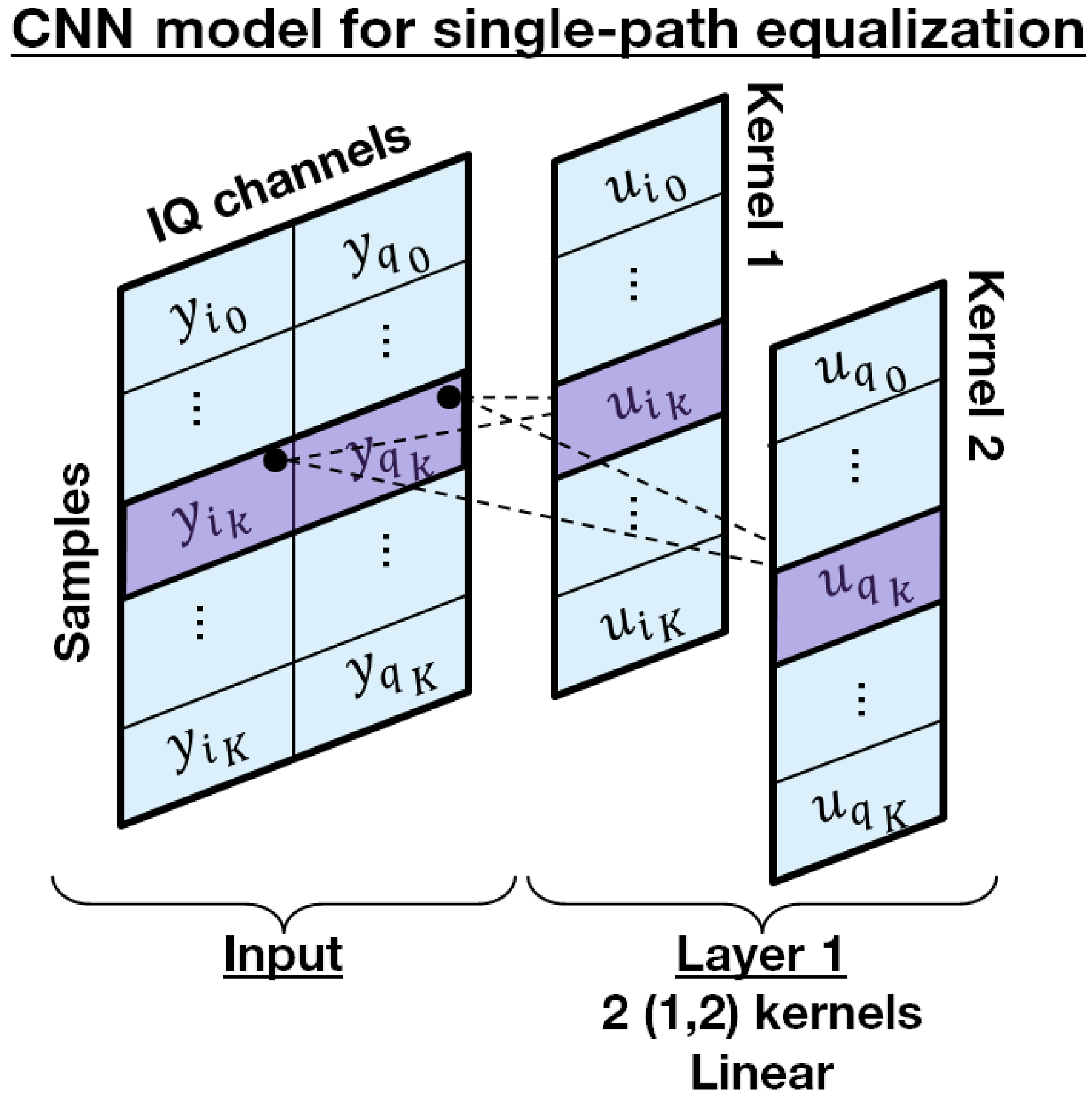
From the optimal equalization scheme presented previously, one can deduce a straightforward NN implementation. The single-path equalization operation can be applied independently to all samples of a given frame affected by the same channel under block-fading hypothesis. A Convolutional Neural Network (CNN) is therefore particularly suited in this case and allows for an efficient parallel processing of samples blocks. The CNN shift invariant architecture, based on shared weights, drastically reduces the number of trainable parameters, independently of the number of samples to process [7]. The proposed minimal CNN to perform single-path equalization consists of one linear layer (
i.e.
without a non-linear activation function) with only two kernels of size \((1,2)\) as described in Figure 2. An input matrix of shape \((K,2)\) is considered, where \(K\) corresponds to the number of samples and \(2\) to real (I channel) and imaginary (Q channel) parts of these samples. The operation performed by such a CNN on a given sample is expressed as:
\[\mathbf{u_k}^{\rm{T}} = \mathbf{y_k}^{\rm{T}}\bf{W} + \mathbf{c}^{\rm{T}} \label{NN_equalizer_output}\]
where \(\mathbf{y_k}\) is the k-th input sample (real and imaginary part of the sample form a vector of two elements) and \(\mathbf{u_k}\) the k-th equalized sample. \(\bf{W}\) and \(\mathbf{c}\) are the \((2\times2)\) weights matrix (each column representing one of the two kernels) and the bias vector of size two, respectively.
Given the optimal solution described in equation [optimal_eq_scheme], the optimal NN parameters are:
\[\label{optimal_NN_weights} \left\{ \begin{aligned} \bf{W}_{\text{optimal}} &= (\bf{RA})^{-1}\\ \mathbf{c}_{\text{optimal}}^{\rm{T}} &= -\mathbf{o}^{\rm{T}}(\bf{RA})^{-1} &\\ \end{aligned} \right.\]
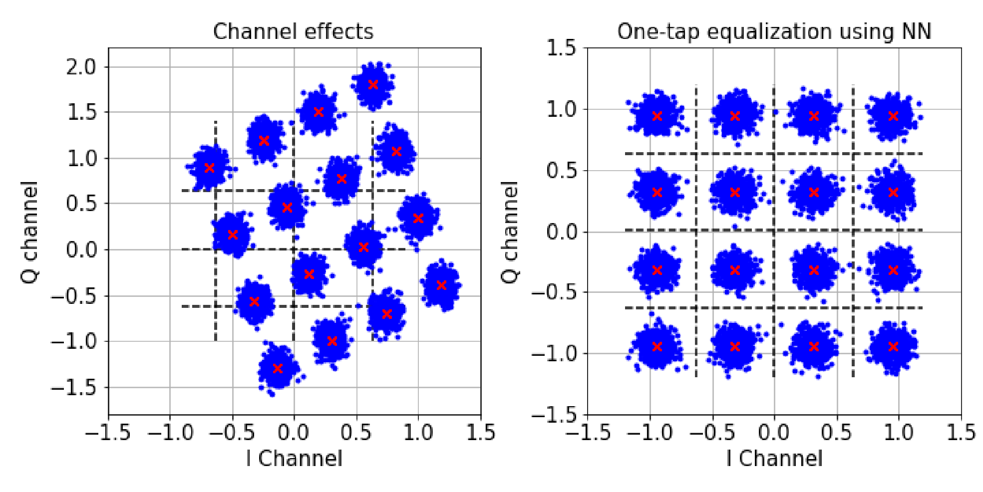
Figure 3 shows the result of the operation applied by this minimal NN to a 16-QAM constellation altered by a channel with arbitrarily defined impairments. One can see that the samples are perfectly equalized.
Designing a NN based detection system
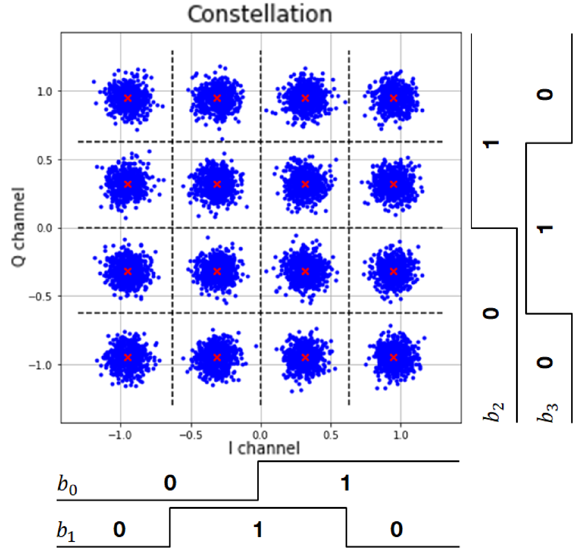
This section describes a minimal NN solving the decision problem faced in a M-QAM demodulator. A demodulation block uses decision boundaries within the complex plane to map noisy samples to symbols, and then to the corresponding binary code-words. The decisions boundaries are chosen to maximize the probability that the detected symbols correspond to the transmitted ones. In the case of a 16-QAM there are six boundaries allowing to distinguish the 16 symbols, as described in the Figure 4.
A NN is known to be efficient to solve the previous decision problem [6], [8]. Indeed, a formal neuron associated with an activation function such as a sigmoid or a Rectified Linear Unit (ReLU) expresses a non-linearity over an hyper-plane as shown in equation [N_output_activation] with the example of ReLU activation. This non-linearity can then be used to define a decision boundary.
\[s = \mathbf{e}^{\rm{T}}\mathbf{w} + c \quad\text{and}\quad \text{ReLU}(s) = \left\{ \begin{aligned} s & \textrm{ if } s>0\\ 0 & \textrm{ otherwise } \end{aligned} \right. \label{N_output_activation}\]
where \(\mathbf{e}\) is the input vector, \(\mathbf{w}\) the weights vector and \(c\) the bias of the neuron. \(s\) is the output of the neuron before activation function, \(\text{ReLU}(s)\) is the output of the neuron after applying the ReLU activation.
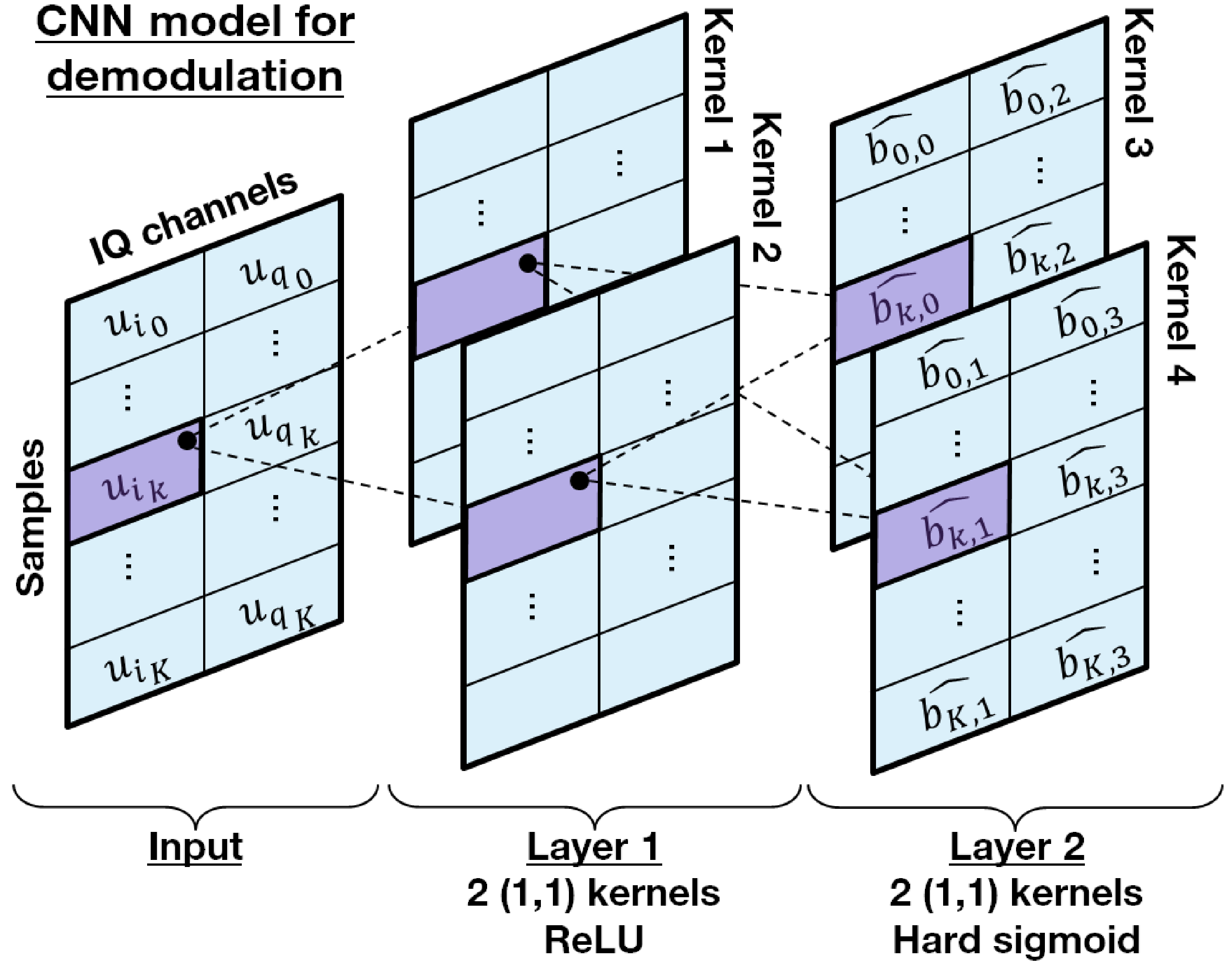
The NN should associate to a sample the corresponding binary code-word. Therefore, the NN need to solve both decision and demapping problems. The proposed model in the case of a 16-QAM, as described in Figure 5, is based on the following observations:
The demodulation operations can be applied independently to each sample. For reasons similar to those described in section 3.1, a CNN with kernels of the size of one sample is particularly well-suited.
The NN carries out both decision and demapping tasks. Following a similar approach to the one proposed in [9], a bit-level decision process is considered instead of symbol-level decision process followed by a symbol-to-bit demapping. The objective of the NN is to approximate the functions stated as \(b_0\),\(b_1\),\(b_2\) and \(b_3\) in Figure 4. Considering the usual monotonic activation functions offered by the majority of NN frameworks, the NN needs at least two layers to compute the desired functions, as \(b_1\) and \(b_3\) aren’t monotonic:
Regarding the input layer, the minimum number of kernels corresponds to the number of decisions boundaries associated to the Least Significant Bit (LSB) on each channel (namely \(b_1\) and \(b_3\)). Consequently, four non-linear kernels are needed (\(2^{\log_{2}(M)/2}\) in the general case of a M-QAM). Considering computational power constraints, ReLU activation is chosen. All the decision boundaries can be expressed as a combination of the four kernels by the output layer.
The output of the NN needs to represent the values of the four bits associated to each symbol. As a result, the output layer needs four kernels (\(\log_{2}(M)\) for a M-QAM). The outputs representing binary values, a sigmoid activation function is particularly well-suited.
Under the assumption that the samples are perfectly equalized, I and Q channels can be processed separately with the same operations, therefore dividing the number and size of the aforementioned kernels by two.
The architecture of this model is scalable to any QAM order by following the number of parameters described in table 1.
| CONVOLUTIONAL LAYER 1 | |
|---|---|
| Input matrix dimensions | \((K,2)\) |
| Kernel number and properties | \(n_1 = 2^{\log_{2}(M)/2-1}\), size \((1,1)\), stride \((1,1)\) |
| Activation | ReLU |
| Output tensor dimensions | \((K,2,n_1)\) |
| CONVOLUTIONAL LAYER 2 | |
| Kernel number and properties | \(n_2 = \log_{2}(M)/2\), size \((1,1)\), stride \((1,1)\) |
| Activation | Hard sigmoid |
| Output tensor dimensions | \((K,2,n_2)\) |
| FLATTEN LAYER | |
| Output vector dimension | \(K\log_{2}(M)\) |
The choice of a hard sigmoid instead of a sigmoid activation on the output layer of the NN is proposed to lower the computational complexity. As shown in equation [hard_sigmoid], the hard sigmoid requires at most two comparisons, one addition and one multiplication.
\[\text{sigmoid}_{\text{hard}}(x) = \left\{ \begin{aligned} & 0 & &\textrm{if } x<-2.5\\ & 1 & &\textrm{if } x>\phantom{-}2.5\\ & 0.2x+0.5 & &\textrm{otherwise} \end{aligned} \right. \label{hard_sigmoid}\]
In the case of 16-QAM, one possible configuration of the weights and bias that is optimal with regard to the theoretical decision boundaries is proposed3:
\[\begin{aligned} &\text{Layer}_{1}\left\{ \begin{aligned} &\mathbf{w}_1 = (-1) & c_1 = 0 \\ &\mathbf{w}_2 = (1) & c_2 = 0 \end{aligned} \right.\\ &\text{Layer}_{2}\left\{ \begin{aligned} &\mathbf{w}_3 = (-1&\phantom{-}1) & &c_3 = 0 \\ &\mathbf{w}_4 = (-1&-1) & &c_4 = 2\delta \end{aligned} \right. \end{aligned}\] where \(\mathbf{w}_i\) and \(c_i\) are respectively the weights vectors and bias of the i-th kernel (following numbering of Figure 5). \(2\delta\) corresponds to the inter-symbol distance of the considered constellation. \(\delta=1/\sqrt{10}\) in the case of a 16-QAM with a power normalized to one.
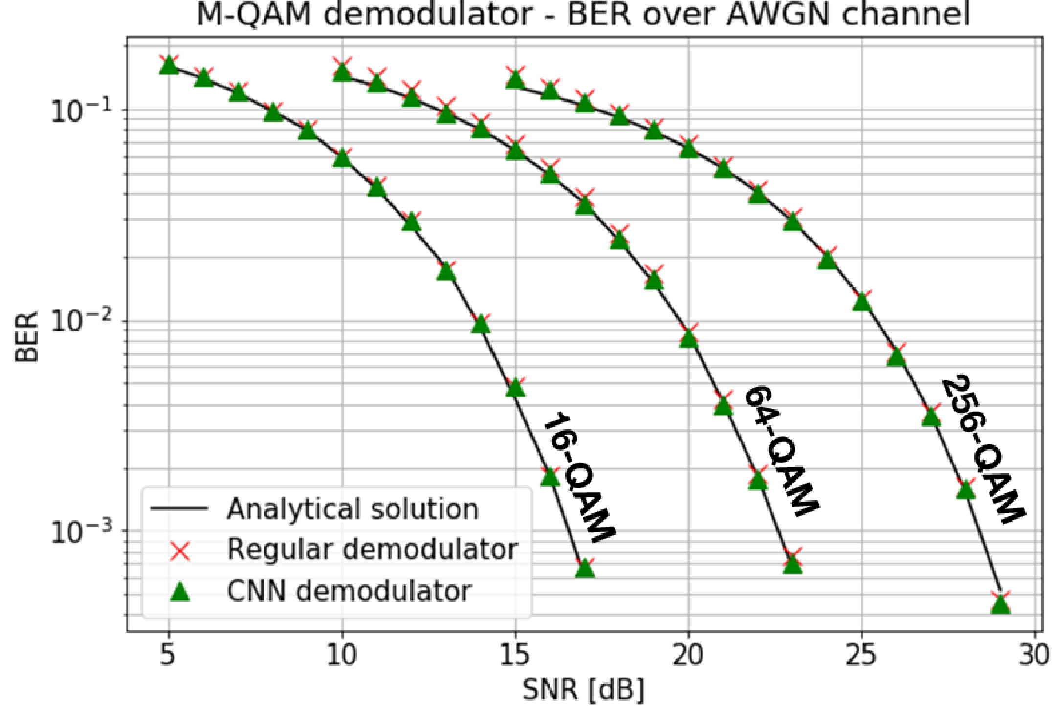
As shown on Figure 6, the proposed model reaches theoretical optimal BER performance4 over AWGN channel for different QAM orders with appropriate configurations of the NN.
As a reference, a demodulator based on minimal Euclidean distance needs \(3M\) additions, \(2M\) multiplications and \(M-1\) comparisons, with \(M\) the order of the QAM modulation[9]. Table 2 presents a comparison in terms of computational complexity between the regular demodulator and the proposed NN model. One can see that the NN outperforms, in terms of complexity, the proposed reference demodulator.
| QAM | Real Multiplications | Real Additions | Real Comparisons | ||||||
|---|---|---|---|---|---|---|---|---|---|
| 2-10 Order | Regular | NN | Improv. | Regular | NN | Improv. | Regular | NN | Improv. |
| (M) | (2M) | Model | (%) | (3M) | Model | (%) | (M-1) | Model | (%) |
| 4 | 8 | 6 | 25 | 12 | 6 | 50 | 3 | 6 | -50 |
| 16 | 32 | 16 | 50 | 48 | 12 | 75 | 15 | 12 | 20 |
| 64 | 128 | 38 | 70 | 192 | 20 | 90 | 63 | 20 | 68 |
| 256 | 512 | 88 | 83 | 768 | 32 | 96 | 255 | 32 | 87 |
| 1024 | 2048 | 202 | 90 | 3072 | 52 | 98 | 1023 | 52 | 95 |
Learning processes
Previous sections propose a mathematical definition of NN architectures and an analytical derivation of their parameters. This section describes the learning processes that can be applied to configure the proposed models. Such process applied to the configuration of the model proposed in section 3.2 is not of particular interest as one can view the demodulation as a deterministic problem (
i.e.
that is not supposed to change over time). On the contrary, it might be interesting to leverage the learning capabilities of NN to continuously adapt the equalization model proposed in section 3.1 to the channel evolution.
To test this approach the channel impairments described in table 3 are considered. The learning algorithm aims to find the weight matrix \(\bf{W}\) and bias vector \(\textbf{c}\) that minimize \(\rm{L_2}\) loss function between the original samples \(x[k]\) and the equalized samples \(u[k]\), as described in Equation [argmin_mse].
| SNR | \(\phi\) | \(\alpha_i\) | \(\alpha_q\) | \(\omega_i\) | \(\omega_q\) |
|---|---|---|---|---|---|
| 20 dB | \(\pi/8\) | \(7.50\rm{e}^{-1}\) | \(1.25\) | \(2.50\rm{e}^{-1}\) | \(2.50\rm{e}^{-1}\) |
\[\underset{\bf{W},\textbf{c}}{\text{Argmin}}\sum_{k}\left(\textbf{x}_k^{\rm{T}}-\textbf{u}_k^{\rm{T}}\right)^2 = \underset{\bf{W},\textbf{c}}{\text{Argmin}}\sum_{k}\left(\textbf{x}_k^{\rm{T}}-\textbf{y}_k^{\rm{T}}\bf{W}+\textbf{c}^{\rm{T}}\right)^2 \label{argmin_mse}\]
After training, the NN parameters are expected to converge toward the optimal solution described in Equation [optimal_NN_weights2]:
\[\left\{ \begin{aligned} \bf{W}_{\text{optimal}} &= (\bf{RA})^{-1} = \begin{pmatrix} 1.23\phantom{\rm{e}^{-1}} & -5.10\rm{e}^{-1} \\ 3.06\rm{e}^{-1} & \phantom{-}7.39\rm{e}^{-1} \end{pmatrix}\\ \mathbf{c}_{\text{optimal}}^{\rm{T}} &= -\mathbf{o}^{\rm{T}}(\bf{RA})^{-1} = \begin{pmatrix} -3.84\rm{e}^{-1}&-5.72\rm{e}^{-2}\\ \end{pmatrix} &\\ \end{aligned} \right. \label{optimal_NN_weights2}\]
A training data-set containing 256 IQ samples is used and the NN is optimized over 50 epochs, using a \(\rm{L_2}\) loss function and Adam optimizer. After training, the NN weights and bias converge closely toward expected values:
\[\left\{ \begin{aligned} \bf{W}_{\text{learned}} &= \begin{pmatrix} 1.21\phantom{\rm{e}^{-1}} & -5,03\rm{e}^{-1}\\ 3.14\rm{e}^{-1} & \phantom{-}7.43\rm{e}^{-1} \end{pmatrix}\\ \mathbf{c}_{\text{learned}}^{\rm{T}} &= \begin{pmatrix} -3.83\rm{e}^{-1}&-5.18\rm{e}^{-2}\\ \end{pmatrix} \end{aligned} \right.\]
A slight bias can be observed in the learned weights. Indeed, MMSE equalizers are known to converge toward a biased solution [10], that can be expressed in the considered case of single-path channel by:
\[\begin{aligned} w_{\rm{MMSE}} = \frac{h^*}{|h|^2+\frac{\mathbb{E}(|n_k|^2)}{\mathbb{E}(|x_k|^2)}} \end{aligned}\] where \(w_{\rm{MMSE}}\) is the complex scalar coefficient of the equalizer that minimizes the \(\rm{L_2}\) loss function between the equalizer output and the expected one (It can be expressed as a \((2\times2)\) real-valued matrix transformation). \(h\) is the complex scalar coefficient of the single-path channel and \(\frac{\mathbb{E}(|n_k|^2)}{\mathbb{E}(|x_k|^2)}\) is the noise to input-signal powers ratio.
Learning process not being the main topic of this paper, the study of this bias and its possible corrections are left for future work.
Experimentation on a SDR test-bed
This section evaluates the performance of the proposed NN based PHY layer in a more realistic situation by using SDR to transmit IQ samples over a controlled AWGN channel, generated by a channel emulator.
Problematic and working assumptions
The objective is to process 16-QAM IQ samples and to realize both single-path equalization and demodulation tasks. The considered signal is constituted of several blocks of symbols, transmitted by an Ettus USRP B210 SDR [11] from TX channel to RX channel through a Spirent Vertex channel emulator [12]. The later adds a controlled amount of Gaussian noise. An unchecked phase shift, considered invariant during the transmission of a block, is also introduced because of the propagation time and the Local Oscillators (LO) misalignment and needs to be corrected by the equalization step. To this end, each block begins with a Zadoff-Chu (ZC) sequence5 of length 256. The ZC sequence is followed by a payload of 4096 16-QAM symbols. On the receiver side, the signal is sampled with an up-sampling factor of 4. The ZC sequence is used as a pilot sequence to identify payload start and ideal sampling instant as well as channel effects. For each block, the detection and synchronization of the payload is performed by a regular maximal correlation based algorithm, but a NN architecture could be envisioned to perform such task. After down-sampling, a ZC sequence of size 256 and a payload of size 4096 are recovered. The objective of the proposed solution is, for each block, to learn the channel effects based on the comparison of the received down-sampled ZC sequence with the theoretical one, and use this knowledge to equalize and demodulate the down-sampled payload.
Proposed NN based solution
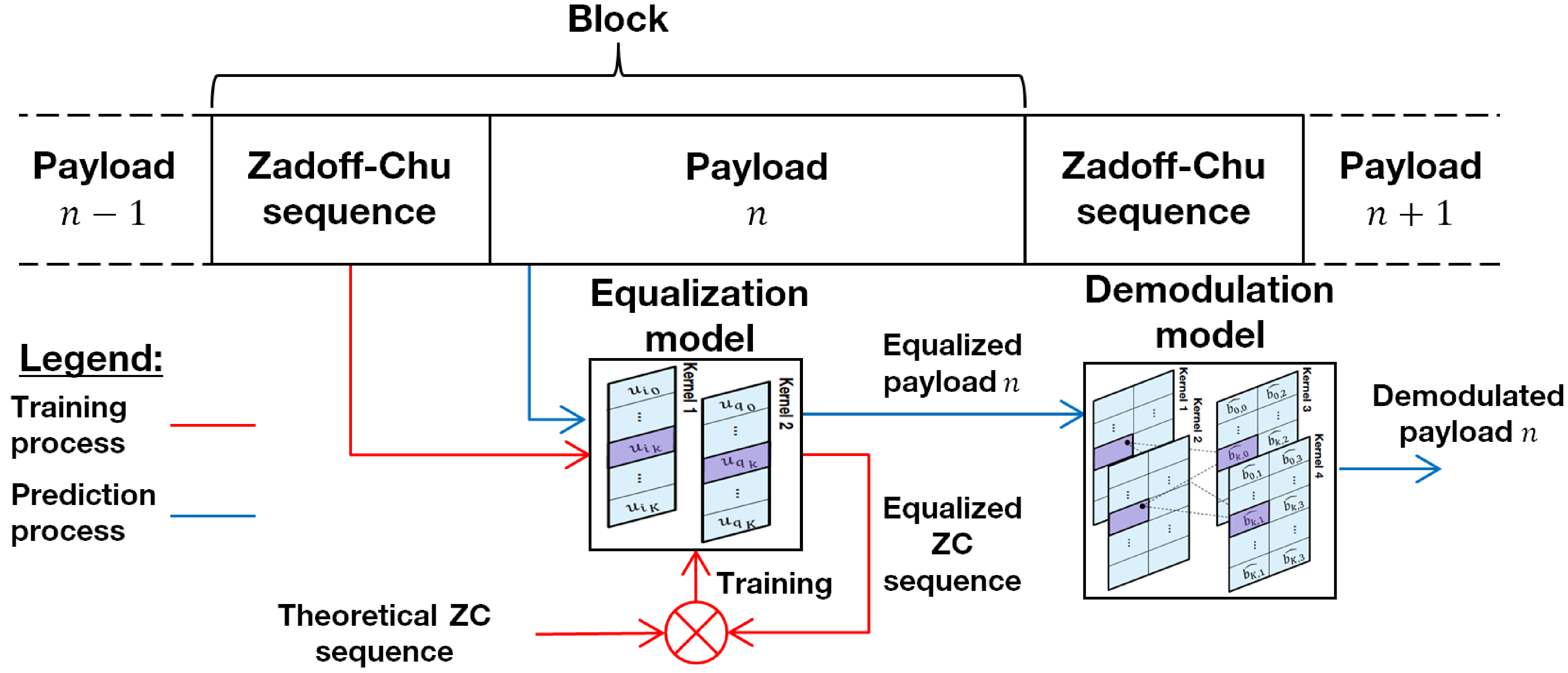
The proposed solution is based on the two NN models introduced in sections 3.1 and 3.2 for equalization and demodulation. The parameters of the demodulation model are set following the configuration proposed in section 3.2. Under the hypothesis of block fading, it is necessary to perform online learning of the equalization model. As described in Figure 7 the proposed system works as follow:
For each block, the equalization model is trained by comparing the received and theoretical ZC sequences. The 256 samples of the ZC sequences are divided in two parts: two third for training and one third for validation. \(\rm{L_2}\) loss and Adam optimizer with a learning rate of 0.1 are used.
After learning, the 4096 IQ samples of the payload are corrected using the newly trained equalization model before being fed to the demodulation model.
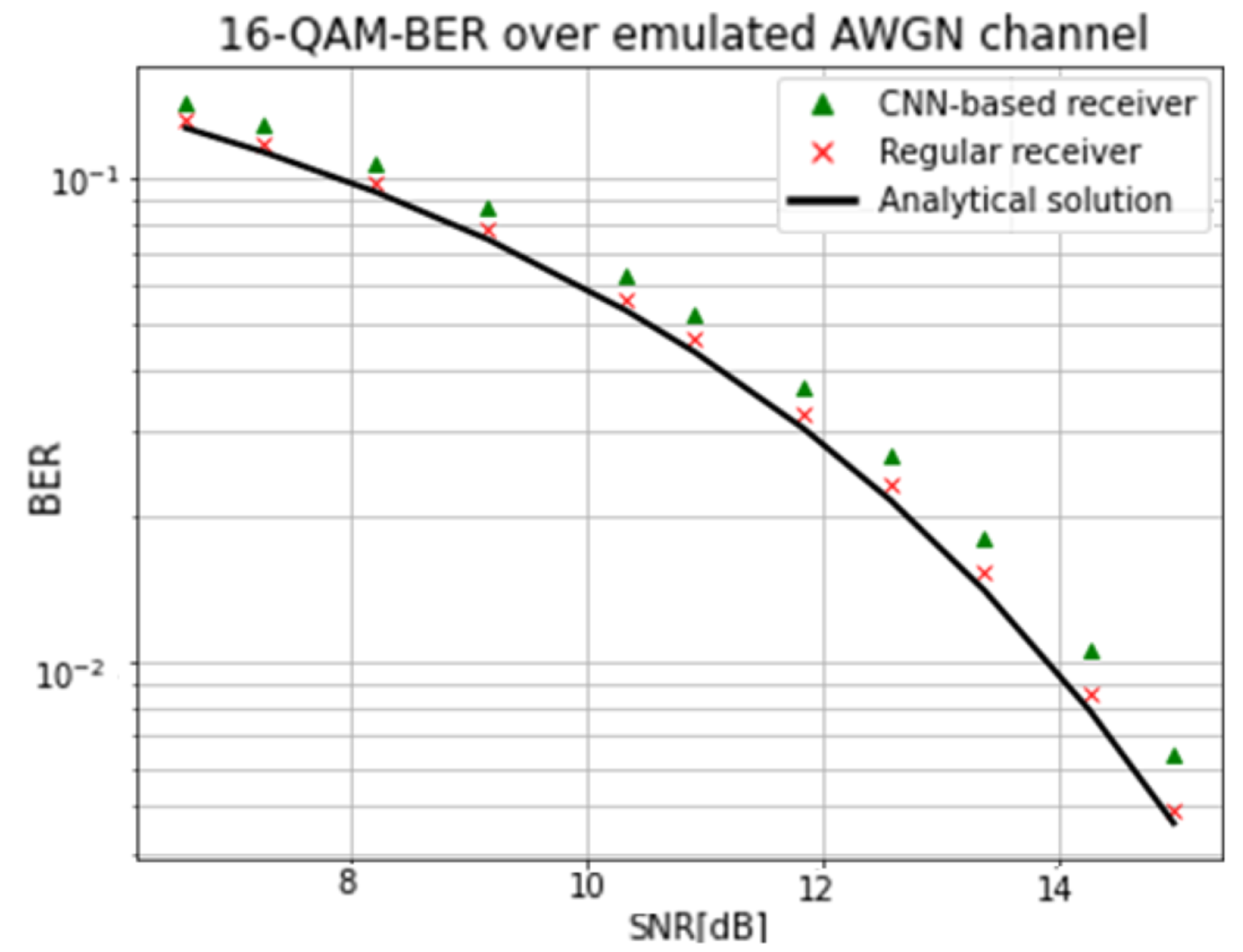
As described in Figure 8, this simple system reaches near optimal BER. As a comparison, the regular receiver estimates the channel parameters by computing the correlation between the received ZC sequence and the theoretical one to perform single-path equalization. A minimal Euclidean distance algorithm is then used for demodulation. One can see a slight degradation of the BER performance of the NN model compared to the regular receiver. This can be explained by the learning bias mentioned in section 4.
Results, Conclusions and perspectives
This paper has described how the problems of single-path equalization and M-QAM demodulation can be expressed in terms of low-complexity NN architectures, relevant with regard to the constraints of IoT systems. The proposed models have been experimentally assessed using SDR based communication chain and a channel emulator, achieving near-optimal performance. Questions related to the training of these minimal models, and notably the question of the learning bias as described in section 4, have not been addressed in depth in this paper and have been left for further publications.
The study of NN complexity is of great importance in the context of 5G and beyond 5G cellular networks for IoT, where it is not always possible to use deep NN. Using low-complexity NN offers the advantages of higher efficiency and reduced learning and inference time. This paper demonstrates that they also mitigate the "black-box" issue that is often criticized in DNN and allow for a better explainability. Moreover, even if low-complexity NN might not be as expressive as their deep counterpart, they still profit of the interesting properties offered by NN dedicated hardware such as Tensor Processing Units (TPU). Indeed, NN are universal approximators [14] but rely on simple individual mathematical operations such as multiplications, additions and basic non-linear activation functions. The expressiveness of NN models lies in their layered architectures and not in complex individual mathematical operations. These properties of NN allow for very efficient and generic hardware to be developed [15]. This hardware generality is interesting in terms of scalability of the PHY layer but also in terms of possible hardware mutualization in a distributed learning and inference scheme or in a Mobile Edge Computing context. Moreover, recent versions of the aforementioned hardware, such as Google Edge TPU, have been developed to address embedded and low power applications. Hence, they are particularly appealing for IoT devices. As more and more companies such as Intel, Nvidia, Apple or Huawei develop NN dedicated hardware, the Total Cost of Ownership (TCO) of NN based communication systems is decreasing. Thus, the more elements of the PHY layer (and beyond) are replaced by NN algorithms, the more one can expect to benefit of the properties described above.
Matrix are denoted as \(\bf{M}\), vector as \(\textbf{v}\) and scalar as \(s\). In this paper, matrix notations are mostly considered instead of complex notations to allow for a direct comparison with the NN real-valued parameters.↩︎
Block-fading hypothesis assumes that the channel coefficients remain constant for a block of \(K\) symbols, depending on the channel coherence time.↩︎
Proposed configuration is not unique and assume a hard demodulation process with a rounding of the output values to either zero or one. Higher dynamic of the output layer parameters might be used to approximate the step function with hard sigmoid activation and avoid rounding the outputs.↩︎
Optimal BER over AWGN channel is computed considering the nearest neighbor approximation and Gray coding.↩︎
Zadoff–Chu sequences are Constant Amplitude Zero Auto-Correlation (CAZAC) wave-forms that exhibits interesting properties [13]. They are notably used in 3GPP LTE and 5G air interfaces.↩︎